User:Marshallsumter/Radiation astronomy2/Radars
Radar astronomy is used to detect and study astronomical objects that reflect radio rays.
The image at right is of asteroid 2012 LZ1 using the Arecibo Planetary Radar.
Radar astronomy is a technique of observing nearby astronomical objects by reflecting microwaves off target objects and analyzing the echoes. Radar astronomy differs from radio astronomy in that the latter is a passive observation and the former an active one. The radar transmission may either be pulsed or continuous.
Radar directly measures the distance to the object (and how fast it is changing). The combination of optical and radar observations normally allows the prediction of orbits at least decades, and sometimes centuries, into the future.
The maximum range of astronomy by radar is very limited, and is confined to the solar system. This is because the signal strength drops off very steeply with distance to the target, the small fraction of incident flux that is reflected by the target, and the limited strength of transmitters.[1] It is also necessary to have a relatively good ephemeris of the target before observing it.
Radars
[edit | edit source]Radio waves are a type of electromagnetic radiation with wavelengths in the electromagnetic spectrum longer than infrared light. Radio waves have frequencies from 300 [Gigahertz] GHz to as low as 3 [Kilohertz] kHz, and corresponding [to] wavelengths from 1 millimeter to 100 kilometers.
| Band name | Frequency range | Wavelength range | Notes |
|---|---|---|---|
| HF | 3–30 MHz | 10–100 m | Coastal radar systems, over-the-horizon radar (OTH) radars; 'high frequency' |
| VHF | 30–300 MHz | 1–10 m | Very long range, ground penetrating; 'very high frequency' |
| P | < 300 MHz | > 1 m | 'P' for 'previous', applied retrospectively to early radar systems; essentially HF + VHF |
| UHF | 300–1000 MHz | 0.3–1 m | Very long range (e.g. ballistic missile early warning), ground penetrating, foliage penetrating; 'ultra high frequency' |
| L | 1–2 GHz | 15–30 cm | Long range air traffic control and surveillance; 'L' for 'long' |
| S | 2–4 GHz | 7.5–15 cm | Moderate range surveillance, Terminal air traffic control, long-range weather, marine radar; 'S' for 'short' |
| C | 4–8 GHz | 3.75–7.5 cm | Satellite transponders; a compromise (hence 'C') between X and S bands; weather; long range tracking |
| X | 8–12 GHz | 2.5–3.75 cm | Missile guidance, marine radar, weather, medium-resolution mapping and ground surveillance; in the USA the narrow range 10.525 GHz ±25 MHz is used for airport radar; short range tracking. Named X band because the frequency was a secret during WW2. |
| Ku | 12–18 GHz | 1.67–2.5 cm | High-resolution, also used for satellite transponders, frequency under K band (hence 'u') |
| K | 18–24 GHz | 1.11–1.67 cm | From German kurz, meaning 'short'; limited use due to absorption by water vapour, so Ku and Ka were used instead for surveillance. K-band is used for detecting clouds by meteorologists, and by police for detecting speeding motorists. K-band radar guns operate at 24.150 ± 0.100 GHz. |
| Ka | 24–40 GHz | 0.75–1.11 cm | Mapping, short range, airport surveillance; frequency just above K band (hence 'a') Photo radar, used to trigger cameras which take pictures of license plates of cars running red lights, operates at 34.300 ± 0.100 GHz. |
| mm | 40–300 GHz | 1.0–7.5 mm | Millimetre band, subdivided as below. The frequency ranges depend on waveguide size. Multiple letters are assigned to these bands by different groups. These are from Baytron, a now defunct company that made test equipment. |
| V | 40–75 GHz | 4.0–7.5 mm | Very strongly absorbed by atmospheric oxygen, which resonates at 60 GHz. |
| W | 75–110 GHz | 2.7–4.0 mm | Used as a visual sensor for experimental autonomous vehicles, high-resolution meteorological observation, and imaging. |
Planetary sciences
[edit | edit source]
"Radar waves penetrate the surface and pass through materials that do not severely attenuate or scatter them. Reflections arise from interfaces with dielectric contrasts. [Shallow radar] SHARAD has penetrated the ∼2-km-thick polar layered deposits in both the north and south, detecting many internal reflectors (17, 18). Smaller targets can be more challenging because SHARAD's antenna pattern is broad, resulting in surface reflections up to a few tens of kilometers away from the suborbital point in rugged areas, versus only a few kilometers in smooth, flat areas. These off-nadir echoes can appear at time delays similar to those arising from subsurface interfaces, so steps are required to avoid misinterpreting this surface clutter as subsurface echoes. Synthetic-aperture data processing is used to improve along-track resolution to ∼300 m, greatly reducing along-track clutter and focusing the surface and subsurface features. We used the known topography of the surface and the radar geometry to model cross-track clutter together with nadir surface echoes [...]. Comparisons of radar sounding data with these synthetic surface echoes and the examination of possible surface echo sources in imagery (19) were undertaken for all cases [...]; such a procedure is a necessary part of radar sounding data interpretation in high-relief environments."[2]
The "Shallow Radar (SHARAD) (15) on the Mars Reconnaissance Orbiter (MRO) to probe the internal structure of several LDAs surrounding massifs on the eastern rim of the Hellas impact basin [first image at the right] where more than 90 LDA complexes flank steep topography (2, 6, 16). The southernmost LDA we studied (LDA-2, [figure at the upper right] has multiple lobes that coalesce to form a continuous deposit extending more than 20 km outward from a massif along ∼170 km of its margins."[2]
"Examination of radar data from SHARAD orbit 6830 where it crosses multiple [lobate debris aprons] LDAs in the eastern Hellas region [...] shows that the only radar reflections not matching simulated surface echoes occur where the spacecraft passes over each LDA [...]; therefore, these echoes are interpreted as arising from within or beneath the LDAs. In one case (LDA-2A), surface clutter is predicted near the terminus of the LDA, where it may obscure portions of a subsurface reflector that clearly extends farther inward below the LDA. LDA-2A and LDA-2B [image at the lower right] show evidence for multiple, closely spaced subsurface reflectors indicating the presence of at least one thin (∼70 m assuming a water-ice composition), distinct deposit below thicker deposits (up to 800 m)."[2]
Theoretical radar astronomy
[edit | edit source]
Here's a couple of theoretical definitions:
Def. the branch of astronomy that uses radar to map the surfaces of planetary bodies in the solar system is called radar astronomy.
Def. reflective and observational astronomy over radio wavelengths is called radar astronomy.
Radiation
[edit | edit source]
Parameters of the array: number of elements - 30, wave length - 10cm, distance between elements - 6.5 cm. The main beam is swept in range [0; PI]. This animation shows range limitations of electronic scanning of phased arrays. There are main lobes of higher orders when a main beam is shifted more than 30 degrees.
Nebulas
[edit | edit source]
The bright lines are a reflection of radar waves upon rain droplets. The eye itself being relatively free of rain is identified by a minimum return of radar energy with the spiral bands of convective cloudiness winding about the eye like a spiral nebula.
Plasmas
[edit | edit source]
There is also a less obvious E-Layer at an altitude of about 110 km. The ionogram clearly shows how the transmitted digisonde signal splits into reflected ordinary and extraordinary waves. The ionogram chart and the parameter FoF2 in the list on the left side of the chart, show that the highest frequency that will be reflected from the ionosphere for vertical incidence (ie., for a radio wave traveling straight up from the ground) is 4.8 MHz.
Aerometeors
[edit | edit source]
On the right is a composite of hourly radar images. These wind gusts averaged ~75 mph over about 450 miles. This is referred to as the Derecho event.
Rocks
[edit | edit source]
The mountain, which has an elevation of 10,948 feet (3,337 meters), is located midway along the lower of the three ridges shown in this radar image from NASA's Cassini spacecraft. Bright regions indicate materials that are rough or that otherwise scatter the beam; dark regions indicate materials that are relatively smooth or that otherwise absorb radar waves. A side effect of this technique is the grainy pattern called "speckle" that typically is present in Cassini radar images.
The fact that Titan has significant mountains at all suggests that some active tectonic forces could be affecting the surface, for example, related to Titan's rotation, tidal forces from Saturn or cooling of the crust.
This radar view was obtained on May 12, 2008 (the flyby called "T-43" by the Cassini team). The image is centered at 2 degrees south latitude, 127 degrees west longitude. The incidence angle is about 34 degrees.
Minerals
[edit | edit source]
Red represents high emissivity and blue low. The image is centered at 12.5S,261E, southeast of Phoebe Regio, Venus and is 587 km on a side. The unnamed volcano is about 2 km high and shows low emissivity at the summit, which could indicate the presence of pyrrohtite or pyrite, minerals which may not be stable at lower altitudes.
Lightnings
[edit | edit source]
Cloud to ground lightning strikes were noted on the National Lightning Detection Network (NLDN) and reported by NWS Buffalo snow spotters during a Lake Effect Snow Storm occurring on the 12 to 13th of October 2006 over the Buffalo (NY) area. While thundersnows themselves are very uncommon (Curran, 1971), those that do occur typically only last up to 5 hours (Market, 2001). The NLDN depicted an average of fifteen cloud to ground strikes per hour between 0000 and 0900 UTC on Oct 13 with fourteen non- consecutive hours of lightning being reported. Here is the 0100 UTC KBUF WSR-88D weather radar composite reflectivity image and National Lightning Detection Network one-hour lightning display : + and - are the lightning strikes, the colors are the snow intensities.
Meteoroids
[edit | edit source]
With a diameter of 11 kilometers (6.8 miles) it is one of the smaller craters on Venus. Because many small meteoroids disintegrate during their passage through the dense atmosphere, there is an absence of craters smaller than 3 kilometers (1.9 miles) in diameter, and even craters smaller than 25 kilometers (15.5 miles) are relatively scarce. The apron of ejected material suggests that the impacting body made contact with the surface from an oblique angle. Upon closer observation it is possible to delineate secondary craters, impact scars from blocks ejected from the primary crater. A feature associated with this and many other Venusian craters is a radar-dark halo. Since dark radar return signifies a smooth surface, it has been hypothesized that an intense shock wave removed or pulverized previously rough surface material or that a blanket of fine material was deposited during or after the impact.
Meteor showers
[edit | edit source]
Total count for the night: 698. Line on the graph annotated with small boxes is the hourly average curve (sum of counts in each 1-hr. period beginning and ending on the half hour). The transmitter is the Air Force Space Surveillance Radar near Olney, Texas. The receiver is the SpaceweatherRadio dot com facility in New Mexico. The geometry is such that the meteors in these counts would have appeared between 10 miles and 40 miles altitude in an arched dome about 100 miles in diameter centered a short distance north of Lubbock, Texas. Update: The IMO "official" peak rate count was ~120/hr.
Fieries
[edit | edit source]
This molten rock is formed in the interior of some planets, including Earth, and some of their satellites. When first erupted from a volcanic vent, lava is a liquid at temperatures from 700 to 1,200 °C (1,292 to 2,192 °F). Up to 100,000 times as viscous as water, lava can flow great distances before cooling and solidifying because of its thixotropic and shear thinning properties.
A lava flow is a moving outpouring of lava, which is created during a non-explosive effusive eruption. When it has stopped moving, lava solidifies to form igneous rock. The term lava flow is commonly shortened to lava. Explosive eruptions produce a mixture of volcanic ash and other fragments called tephra, rather than lava flows. The word "lava" comes from Italian, and is probably derived from the Latin word labes which means a fall or slide. The first use in connection with extruded magma (molten rock below the Earth's surface) was apparently in a short account written by Francesco Serao on the eruption of Vesuvius between May 14 and June 4, 1737. Serao described "a flow of fiery lava" as an analogy to the flow of water and mud down the flanks of the volcano following heavy rain.
ʻAʻā is one of three basic types of flow lava. ʻAʻā is basaltic lava characterized by a rough or rubbly surface composed of broken lava blocks called clinker.
The loose, broken, and sharp, spiny surface of an ʻaʻā flow makes hiking difficult and slow. The clinkery surface actually covers a massive dense core, which is the most active part of the flow. As pasty lava in the core travels downslope, the clinkers are carried along at the surface. At the leading edge of an ʻaʻā flow, however, these cooled fragments tumble down the steep front and are buried by the advancing flow. This produces a layer of lava fragments both at the bottom and top of an ʻaʻā flow.
Accretionary lava balls as large as 3 metres (10 feet) are common on ʻaʻā flows. ʻAʻā is usually of higher viscosity than pāhoehoe. Pāhoehoe can turn into ʻaʻā if it becomes turbulent from meeting impediments or steep slopes.
The sharp, angled texture makes ʻaʻā a strong radar reflector, and can easily be seen from an orbiting satellite (bright on Magellan pictures).
ʻAʻā lavas typically erupt at temperatures of 1000 to 1100 °C.
Particles
[edit | edit source]
The image shows long, dark ridges similar to those seen in previous flybys. These are interpreted to be longitudinal dunes. Dunes are mostly an equatorial phenomenon on Titan, and the material forming them may be solid organic particles or ice coated with organic material. Spaced up to 3 kilometers (about 2 miles) apart, these dunes curve around bright features that may be high-standing topographic obstacles, in conformity with the wind patterns. The interaction between the two types of features is complex and not well understood, but clearly the topography and the dunes have influenced each other in other ways as well.
This image is centered at 44 degrees west longitude, 8 degrees north latitude and covers approximately 160 by 325 kilometers (99 by 202 miles) on Titan's surface. The smallest details in this image are about 500 meters (about 550 yards) across.
Cryometeors
[edit | edit source]
On the right is a radarsat image of ice streams flowing into the Filchner-Ronne ice shelf. Annotations outline the Rutford ice stream.
Glaciers
[edit | edit source]
On the right is a radar image of Alfred Ernest Ice Shelf on Ellesmere Island, taken by the ERS-1 satellite.
Glaciology
[edit | edit source]
"A small island obstructs the constant flow of the ice shelf on Queen Maud Land – it is the lighter area at the bottom left of the image [on the right]. From September 2010 until it broke off, Iceberg A 62 was connected to the Fimbul Ice Shelf by a mere 800-metre-wide bridge. Two fissures in the ice from different sides of the bridge approached one another until the break occurred. The images transmitted by the radar satellite TerraSAR-X over a long period of time should enable researchers to achieve a better understanding of how icebergs calve."[3]
Hydrometors
[edit | edit source]
On the right, the Quill satellite radar image is shown of the flooded Eel River outflow current debris field in gray.
"Colored content is USGS-derived base map. Gray overlay is derived from a "Quill" satellite radar image made during the December 1964 flooding of California's Eel River. Accurate registration of the overlay onto the map is demonstrated by the excellent match of the stream-valley features in each."[4]
Opticals
[edit | edit source]
Smoothed and contour-filled optical albedo map of Viikinkoski et al. (2018) and Ferrais et al. (2020) with purported topographical and albedo features labeled. Approximate outlines of depressions Eros, Foxtrot, and Panthia are indicated with dashed lines. Indeterminate features are indicated with a label and question mark. The subradar centers of each calibrated radar echo are shown. Optical albedo is shown as multiplicative deviations from the mean (pv = 0.16 with a range of 0.13–0.19). Three additional optical bright spots noted by Ferrais et al. are indicated with stylized white symbols.
By optical astronomy, optical observations measure very accurately where an object appears on the sky, but cannot measure the distance accurately at all.
Craters
[edit | edit source]


On the right is a synthetic aperture radar image of the Haughton impact crater on Devon Island, Nunavut, Canada.
On the left is a topographic map from Shuttle Radar Topography Mission data of Iturralde Crater, an unconfirmed impact crater in Bolivia.
Second down on the right: "This figure shows a comparison of interferograms from four different years mapping the rapid ground subsidence over the Lost Hills oil field in California. Lost Hills is located about 60 km (40 miles) northwest of Bakersfield in the San Joaquin Valley. The oil field is about 1.5 km (1mile) wide and 6 km (3.5 miles) long."[5]
"Each interferogram was created using pairs of images taken by synthetic aperture radar that have been combined to measure surface deformation or changes that may have occurred in the time between when data for the two images were taken. The images were collected by the European Space Agency's Remote Sensing satellites (ERS-1 and ERS-2) in two months of each year shown (1995, 1996, 1998 and 1999) and were combined to produce these image maps of the apparent surface deformation, or changes."[5]
"The interferometric measurements that show the changes, primarily vertical subsidence of the surface, are rendered in color with purple indicating no motion and the brightest red showing rapid subsidence. The white areas are where the radar measurements could not be obtained, mostly in the agricultural fields around the oil fields where plant growth or plowing altered the radar properties of the surface."[5]
"These radar data show that parts of the oil field were subsiding unusually rapidly, more than 3 centimeters (1.2 inches) a month, in 1995 and 1996. They also reveal that while the ground subsidence rate decreased in the center part of the oil field, it increased in the northern part between 1995 and 1996 and 1998 and 1999."[5]
Active faults
[edit | edit source]
"Earthquake faults commonly lie between the mountains and the lowlands. The San Andreas fault, the largest fault in California, likewise divides the very rugged San Gabriel Mountains from the low-relief Mojave Desert, thus forming a straight topographic boundary between the top center and lower right corner of the image. We present two versions of this perspective image from NASA's Shuttle Radar Topography Mission (SRTM): one with and one without a graphic overlay that maps faults that have been active in Late Quaternary times (white lines). The fault database was provided by the U.S. Geological Survey."[6]
"The Landsat image used here was acquired on May 4, 2001, about seven weeks before the summer solstice, so natural terrain shading is not particularly strong. It is also not especially apparent given a view direction (northwest) nearly parallel to the sun illumination (shadows generally fall on the backsides of mountains). Consequently, topographic shading derived from the SRTM elevation model was added to the Landsat image, with a false sun illumination from the left (southwest). This synthetic shading enhances the appearance of the topography."[6]
"Landsat has been providing visible and infrared views of the Earth since 1972. SRTM elevation data matches the 30-meter (98-foot) resolution of most Landsat images and substantially helps in analyzing the large and growing Landsat image archive. This Landsat 7 Thematic Mapper image was provided to the SRTM project by the United States Geological Survey, Earth Resources Observation Systems (EROS) Data Center, Sioux Falls, S.D."[6]
"Elevation data used in this image was acquired by the SRTM aboard the Space Shuttle Endeavour, launched on Feb. 11, 2000. SRTM used the same radar instrument that comprised the Spaceborne Imaging Radar-C/X-Band Synthetic Aperture Radar (SIR-C/X-SAR) that flew twice on the Space Shuttle Endeavour in 1994. SRTM was designed to collect 3-D measurements of the Earth's surface. To collect the 3-D data, engineers added a 60-meter (approximately 200-foot) mast, installed additional C-band and X-band antennas, and improved tracking and navigation devices. The mission is a cooperative project between NASA, the National Imagery and Mapping Agency (NIMA) of the U.S. Department of Defense and the German and Italian space agencies."[6]
"Size: View width 134 kilometers (83 miles); view distance 150 kilometers (93 miles) Location: 34.3 degrees North latitude, 118.4 degrees West longitude Orientation: View west-northwest, 1.8 X vertical exaggeration Image Data: Landsat Bands 3, 2+4, 1 as red, green, blue, respectively Original Data Resolution: SRTM 1 arcsecond (30 meters or 98 feet), Landsat 30 meters (98 feet) Graphic Data: earthquake faults active in Late Quaternary times Date Acquired: February 2000 (SRTM), May 4, 2001 (Landsat)."[6]
Transform faults
[edit | edit source]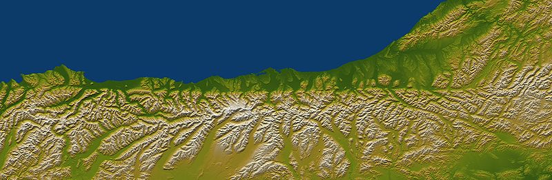
"The Alpine fault runs parallel to, and just inland of, much of the west coast of New Zealand's South Island. This view was created from the near-global digital elevation model produced by the Shuttle Radar Topography Mission (SRTM) and is almost 500 kilometers (just over 300 miles) wide. Northwest is toward the top. The fault is extremely distinct in the topographic pattern, nearly slicing this scene in half lengthwise."[7]
"In a regional context, the Alpine fault is part of a system of faults that connects a west dipping subduction zone to the northeast with an east dipping subduction zone to the southwest, both of which occur along the juncture of the Indo-Australian and Pacific tectonic plates. Thus, the fault itself constitutes the major surface manifestation of the plate boundary here. Offsets of streams and ridges evident in the field, and in this view of SRTM data, indicate right-lateral fault motion. But convergence also occurs across the fault, and this causes the continued uplift of the Southern Alps, New Zealand's largest mountain range, along the southeast side of the fault."[7]
"Two visualization methods were combined to produce this image: shading and color coding of topographic height. The shade image was derived by computing topographic slope in the northwest-southeast (image top to bottom) direction, so that northwest slopes appear bright and southeast slopes appear dark. Color coding is directly related to topographic height, with green at the lower elevations, rising through yellow and tan, to white at the highest elevations."[7]
"Elevation data used in this image were acquired by the Shuttle Radar Topography Mission aboard the Space Shuttle Endeavour, launched on Feb. 11, 2000. SRTM used the same radar instrument that comprised the Spaceborne Imaging Radar-C/X-Band Synthetic Aperture Radar (SIR-C/X-SAR) that flew twice on the Space Shuttle Endeavour in 1994. SRTM was designed to collect 3-D measurements of the Earth's surface. To collect the 3-D data, engineers added a 60-meter (approximately 200-foot) mast, installed additional C-band and X-band antennas, and improved tracking and navigation devices."[7]
The Alpine fault is "495 kilometers (307 miles) by 162 kilometers (100 miles). Location: 43.2 degrees South latitude, 170.5 degrees East longitude. Orientation: Northwest toward the top".[7]
Volcanoes
[edit | edit source]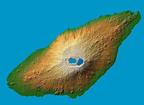

"The recently active volcano Mt. Manaro is the dominant feature in this shaded relief image [on the right] of Ambae Island, part of the Vanuatu archipelago located 1400 miles northeast of Sydney, Australia. About 5000 inhabitants, half the island's population, were evacuated in early December from the path of a possible lahar, or mud flow, when the volcano started spewing clouds of steam and toxic gases 10,000 feet into the atmosphere."[8]
"Last active in 1996, the 1496 meter (4908 ft.) high Hawaiian-style basaltic shield volcano features two lakes within its summit caldera, or crater. The ash and gas plume is actually emerging from a vent at the center of Lake Voui (at left), which was formed approximately 425 years ago after an explosive eruption."[8]
"Two visualization methods were combined to produce the image: shading and color coding of topographic height. The shade image was derived by computing topographic slope in the northwest-southeast direction, so that northwest slopes appear bright and southeast slopes appear dark. Color coding is directly related to topographic height, with green at the lower elevations, rising through yellow and tan, to white at the highest elevations."[8]
"Elevation data used in this image were acquired by the Shuttle Radar Topography Mission [SRTM] aboard the Space Shuttle Endeavour, launched on Feb. 11, 2000. SRTM used the same radar instrument that comprised the Spaceborne Imaging Radar-C/X-Band Synthetic Aperture Radar (SIR-C/X-SAR) that flew twice on the Space Shuttle Endeavour in 1994. SRTM was designed to collect 3-D measurements of the Earth's surface. To collect the 3-D data, engineers added a 60-meter (approximately 200-foot) mast, installed additional C-band and X-band antennas, and improved tracking and navigation devices."[8]
"Location: 15.4 degree south latitude, 167.9 degrees east longitude; Orientation: North toward the top, Mercator projection; Size: 36.8 by 27.8 kilometers (22.9 by 17.3 miles); Image Data [is a] shaded and colored SRTM elevation model"[8]
On the left is a space radar image of Klyuchevskaya sopka.
"This is an image of the area of the Kliuchevskoi volcano, Kamchatka, Russia, which began to erupt on September 30, 1994. Kliuchevskoi is the blue triangular peak in the center of the image, towards the left edge of the bright red area that delineates bare snow cover. The image was acquired by the Spaceborne Imaging Radar-C/X-Band Synthetic Aperture Radar (SIR-C/X-SAR) aboard the space shuttle Endeavour on its 88th orbit on October 5, 1994. The image shows an area approximately 75 kilometers by 100 kilometers (46 miles by 62 miles) that is centered at 56.07 degrees north latitude and 160.84 degrees east longitude. North is toward the bottom of the image. The radar illumination is from the top of the image. The Kamchatka volcanoes are among the most active volcanoes in the world. The volcanic zone sits above a tectonic plate boundary, where the Pacific plate is sinking beneath the northeast edge of the Eurasian plate. The Endeavour crew obtained dramatic video and photographic images of this region during the eruption [...]. The colors in this image were obtained using the following radar channels: red represents the L-band, HH (horizontally transmitted and received) channel; green represents the L-band, HV (horizontally transmitted and vertically received) channel; blue represents the C-band, HV (horizontally transmitted and vertically received) channel. In addition to Kliuchevskoi, two other active volcanoes are visible in the image. Bezymianny, the circular crater above and to the right of Kliuchevskoi, contains a slowly growing lava dome. Tolbachik is the large volcano with a dark summit crater near the upper right edge of the red snow covered area. The Kamchatka River runs from right to left across the bottom of the image. The 1994 eruption of Kliuchevskoi included massive ejections of gas, vapor and ash, which reached altitudes of 15,000 meters (50,000 feet). Melting snow mixed with volcanic ash triggered mud flows on the flanks of the volcano. Paths of these flows can be seen as thin lines in various shades of blue and green on the north flank in the center of the image."[9]
Mercury
[edit | edit source]
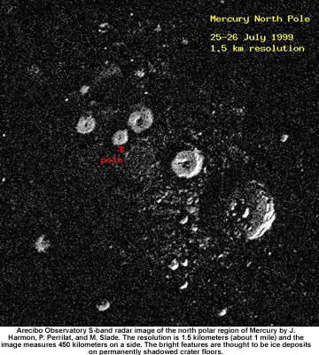
Radar astronomy of Mercury improved the value for the distance from the earth including the rotational period, libration,[and surface mapping, especially of the polar regions.
In "1991, [...] the Arecibo radio telescope in Puerto Rico detected unusually radar-bright patches at Mercury's poles, spots that reflected radio waves in the way one would expect if there were water ice [denoted in the image at right by yellow areas]. Many of these patches corresponded to the location of large impact craters mapped by the Mariner 10 spacecraft in the 1970s."[10]
"Images from the spacecraft's Mercury Dual Imaging System taken in 2011 and earlier this year confirmed that radar-bright features at Mercury's north and south poles are within shadowed regions on Mercury's surface, findings that are consistent with the water-ice hypothesis."[10]
"The neutron data indicate that Mercury's radar-bright polar deposits contain, on average, a hydrogen-rich layer more than tens of centimeters thick beneath a surficial layer 10 to 20 centimeters thick that is less rich in hydrogen".[11]
"The buried layer has a hydrogen content consistent with nearly pure water ice."[11]
"These reflectance anomalies are concentrated on poleward-facing slopes and are spatially collocated with areas of high radar backscatter postulated to be the result of near-surface water ice".[12]
"Correlation of observed reflectance with modeled temperatures indicates that the optically bright regions are consistent with surface water ice."[12]
MESSENGER's Mercury Laser Altimeter (MLA) data "show that the spatial distribution of regions of high radar backscatter is well matched by the predicted distribution of thermally stable water ice".[13]
Water ice strongly reflects radar, and observations by the 70 m [Goldstone Deep Space Communications Complex] Goldstone telescope and the [Very Large Array] VLA in the early 1990s revealed that there are patches of very high radar reflection near the poles.[14] While ice is not the only possible cause of these reflective regions, astronomers believe it is the most likely.[15]
Venus
[edit | edit source]

The first un-ambiguous detection of Venus was made by the Jet Propulsion Laboratory (JPL) on 10 March 1961. A correct measurement of the AU soon followed.
"The advantages of radar in planetary astronomy result from (1) the observer's control of all the attributes of the coherent signal used to illuminate the target, especially the wave form's time/frequency modulation and polarization; (2) the ability of radar to resolve objects spatially via measurements of the distribution of echo power in time delay and Doppler frequency; (3) the pronounced degree to which delay-Doppler measurements constrain orbits and spin vectors; and (4) centimeter-to-meter wavelengths, which easily penetrate optically opaque planetary clouds and cometary comae, permit investigation of near-surface macrostructure and bulk density, and are sensitive to high concentrations of metal or, in certain situations, ice."[16]
The radar image at left shows that just beneath the cloud layers is a rocky object.
Earth
[edit | edit source]

Numerous airborne and spacecraft radars have mapped the entire planet, for various purposes. One example is the Shuttle Radar Topography Mission, which mapped the entire Earth at 30 m resolution.
"The impact of an asteroid or comet several hundred million years ago left scars in the landscape that are still visible in this spaceborne radar image [on the right] of an area in the Sahara Desert of northern Chad. The concentric ring structure is the Aorounga impact crater, with a diameter of about 17 kilometers (10.5 miles). The original crater was buried by sediments, which were then partially eroded to reveal the current ring-like appearance. The dark streaks are deposits of windblown sand that migrate along valleys cut by thousands of years of wind erosion. The dark band in the upper right of the image is a portion of a proposed second crater."[17]
"Radar imaging is a valuable tool for the study of desert regions because the radar waves can penetrate thin layers of dry sand to reveal details of geologic structure that are invisible to other sensors. The image was acquired by the Spaceborne Imaging Radar-C/X-band Synthetic Aperture Radar (SIR-C/X-SAR) on April 18 and 19, 1994, onboard the space shuttle Endeavour. The area shown is 22 kilometers by 28 kilometers (14 miles by 17 miles) and is centered at 19.1 degrees north latitude, 19.3 degrees east longitude. North is toward the upper right. The colors are assigned to different radar frequencies and polarizations as follows: red is L-band, horizontally transmitted and received; green is C-band, horizontally transmitted and received; and blue is C-band, horizontally transmitted, vertically received."[17]
At right is a shaded relief map of Antarctica developed from RADARSAT Synthetic Aperture Radar data. RADARSAT is a Canadian satellite.
Moon
[edit | edit source]


The moon is comparatively close and was detected by radar, soon after the invention of the technique, in 1946.[18][19] Measurements included surface roughness and later mapping of shadowed regions near the poles.
"Clementine orbited the Moon in 1994 for 71 days, mapping the Moon globally in 11 wavelengths and measuring its topography by laser ranging. [... The] bistatic radar experiment (so-called because the spacecraft transmitted while we listened to the echoes on Earth) found evidence in the dark areas near the south pole of the Moon for material with high circular polarization ratio [CPR]".[20]
"Meanwhile, astronomers on Earth began publishing results questioning the Clementine and Lunar Prospector [1998-2000] results. With the giant Arecibo radiotelescope, radar images were taken from the Earth. They found radar reflections with high CPR lying in both permanent darkness and in sunlit areas. Ice is not stable in sunlight, so they postulated that all high CPR is caused by surface roughness; if any ice is at the lunar poles, it must be in a finely disseminated form, invisible to radar mapping."[20]
The experiment from Clemintine "was bistatic, i.e., the transmitter and receiver were in different places. Bistatic radar has the advantage of observing reflections through the phase angle, the angle between transmitted and received radio rays [...]. This phase dependence is important. It’s similar to the effect one gets from looking at a bicycle reflector at just the right angle: at certain angles, the internal planes in the transparent plastic align and a very bright reflection is seen. Similarly, in both radio and visible wavelengths on the Moon, we see an “opposition surge”, an apparent increase in brightness looking directly down from the sun (zero phase). Clementine orbited the Moon such that we could observe its phase dependence [...] and we specifically looked for this “opposition surge”, called the Coherent Backscatter Opposition Effect (CBOE). CBOE is particularly valuable to identify ice on planetary surfaces."[20]
"Clementine transmitted right circular polarized (RCP) radio and we listened on Earth in both right- and left-circular polarized (LCP) channels. The ratio of power received in these two channels is called the circular polarization ratio (CPR). The dry, equatorial Moon has CPR less than one, but the icy satellites of Jupiter all have CPR greater than one. We know these objects have surfaces of water ice; in this case, the ice acts as a radio-transparent media in which waves penetrate the ice, are scattered and reflected multiple times, and returned such that some of the waves are received in the same polarization sense as they are sent—they have CPR greater than unity"[20]
"The problem with CPR alone is that we can also get high values from very rough surfaces, such as a rough, blocky lava flow, which has angles that form many small corner reflectors. In this case, a radio wave could hit a rock face (changing RCP into LCP) and then bounce over to another rock face (changing the LCP back into RCP) and hence to the receiver [...]. This “double-bounce” effect also creates high CPR in that “same sense” reflections could mimic the enhanced CPR one gets from ice targets."[20]
At lower right is an image using the Goldstone DSS-14 antenna as a transmitter and the DSS-13 as a receiver, a form of radar interferometry. The cross for the south pole in the Arecibo image is in the Shackleton crater of the Goldstone image.
"Very precise microwave measurements between two spacecraft, named Ebb and Flow, were used to map gravity with high precision and high spatial resolution. The field shown resolves blocks on the surface of about 12 miles (20 kilometres) and measurements are three to five orders of magnitude improved over previous data. Red corresponds to mass excesses and blue corresponds to mass deficiencies. The map shows more small-scale detail on the far side of the moon compared to the nearside because the far side has many more small craters."[21]
"Twin NASA probes orbiting Earth's moon have generated the highest resolution gravity field map of any celestial body. The new map, created by the Gravity Recovery and Interior Laboratory (GRAIL) mission, is allowing scientists to learn about the moon's internal structure and composition in unprecedented detail. Data from the two washing machine-sized spacecraft also will provide a better understanding of how Earth and other rocky planets in the solar system formed and evolved."[21]
"The gravity field map reveals an abundance of features never before seen in detail, such as tectonic structures, volcanic landforms, basin rings, crater central peaks and numerous simple, bowl-shaped craters. Data also show the moon's gravity field is unlike that of any terrestrial planet in our solar system."[22]
""What this map tells us is that more than any other celestial body we know of, the moon wears its gravity field on its sleeve," said GRAIL Principal Investigator Maria Zuber of the Massachusetts Institute of Technology in Cambridge. "When we see a notable change in the gravity field, we can sync up this change with surface topography features such as craters, rilles or mountains.""[22]
"According to Zuber, the moon's gravity field preserves the record of impact bombardment that characterized all terrestrial planetary bodies and reveals evidence for fracturing of the interior extending to the deep crust and possibly the mantle. This impact record is preserved, and now precisely measured, on the moon. The probes revealed the bulk density of the moon's highland crust is substantially lower than generally assumed. This low-bulk crustal density agrees well with data obtained during the final Apollo lunar missions in the early 1970s, indicating that local samples returned by astronauts are indicative of global processes."[22]
""With our new crustal bulk density determination, we find that the average thickness of the moon's crust is between 21 and 27 miles (34 and 43 kilometres), which is about 6 to 12 miles (10 to 20 kilometres) thinner than previously thought," said Mark Wieczorek, GRAIL co-investigator at the Institut de Physique du Globe de Paris. "With this crustal thickness, the bulk composition of the moon is similar to that of Earth. This supports models where the moon is derived from Earth materials that were ejected during a giant impact event early in solar system history.""[22]
"The map was created by the spacecraft transmitting radio signals to define precisely the distance between them as they orbit the moon in formation. As they fly over areas of greater and lesser gravity caused by visible features, such as mountains and craters, and masses hidden beneath the lunar surface, the distance between the two spacecraft will change slightly."[22]
""We used gradients of the gravity field in order to highlight smaller and narrower structures than could be seen in previous datasets," said Jeff Andrews-Hanna, a GRAIL guest scientist with the Colorado School of Mines in Golden. "This data revealed a population of long, linear gravity anomalies, with lengths of hundreds of kilometres, crisscrossing the surface. These linear gravity anomalies indicate the presence of dikes, or long, thin, vertical bodies of solidified magma in the subsurface. The dikes are among the oldest features on the moon, and understanding them will tell us about its early history.""[22]
At fourth right is an image of the Moon using its thermal emission at 850 microns.
"The Moon and planets are not detectable by reflected solar radiation at radio wavelengths. However, they all emit thermal radiation, and Jupiter is a strong nonthermal source as well. If the Sun were suddenly switched off, the planets would remain radio sources for a long time, slowly fading as they cooled. At first glance, the λ = 0.85 mm radio image of the Moon [at second right] looks familiar, but there are differences from the visible Moon."[23]
"The darker right edge of the Moon is not being illuminated by the Sun, but it still emits radio waves because it does not cool to absolute zero during the lunar night. A subtler point is that the radio emission is not produced at the visible surface; it emerges from a layer about ten wavelengths thick. As a result, monthly temperature variations of the Moon decrease with increasing wavelength. These wavelength-dependent temperature variations encode information about the conductivity and heat capacity of the rocky and dusty outer layers of the Moon."[23]
"Radar images like the one [at fifth right] were recently used to search for water ice trapped in cold craters near the lunar poles."[23]
The ESA Lunar Lander Mission Lunar Dust Environment and Plasma Package: "Observe radio spectrum (with an additional goal to prepare for future radiation astronomy activities.)"[24]
Mars
[edit | edit source]

Mapping of surface roughness [has been performed] from Arecibo Observatory. The Mars Express mission carries a ground-penetrating radar.
The image at right "shows a cross-section of a portion of the north polar ice cap of Mars, derived from data acquired by the Mars Reconnaissance Orbiter's Shallow Radar (SHARAD), one of six instruments on the spacecraft. The data depict the region's internal ice structure, with annotations describing different layers. The ice depicted in this graphic is approximately 2 kilometers (1.2 miles) thick and 250 kilometers (155 miles) across. White lines show reflection of the radar signal back to the spacecraft. Each line represents a place where a layer sits on top of another. Scientists study how thick the pancake-like layers are, where they bulge and how they tilt up or down to understand what the surface of the ice sheet was like in the past as each new layer was deposited."[25]
The image at left, "called an ionogram, shows data from sounding Mars' ionosphere with the Mars Advanced Radar for Subsurface and Ionospheric Sounding (MARSIS). The horizontal axis is the frequency of the pulse. The left vertical axis is the time delay after transmitting the pulse, with time increasing downward. The right vertical axis is a conversion of time delay to distance, showing the apparent range to the reflection point. The intensity of the received signal at any given frequency and apparent range is indicated by the color, with dark blue being the least intense and green being the most intense."[26]
"The green echo at an apparent range of about 800 kilometers (497 miles) from 2.5 to 5.5 megahertz is the reflected signal from the surface of Mars. The curved bright green feature with an apparent range varying from about 600 to 750 kilometers (373 to 466 miles) at frequencies from about 0.7 to 1.8 megahertz is the echo from the top side of the ionosphere. A second echo of the ionosphere, at an apparent range of about 100 kilometers (62 miles) is labeled "Oblique ionospheric echo." Such echoes are believed to come from distorted structures in the ionosphere caused by the magnetic fields in the crust of Mars."[26]
"MARSIS is an instrument on the European Space Agency's Mars Express orbiter."[26]
At lower right is a "radargram from the Shallow Subsurface Radar instrument (SHARAD)".[27]
The "Shallow Subsurface Radar instrument (SHARAD) on NASA's Mars Reconnaissance Orbiter [radargram] is shown in the upper-right panel and reveals detailed structure in the polar layered deposits of the south pole of Mars."[27]
"The sounding radar collected the data presented here during orbit 1334 of the mission, on Nov. 8, 2006."[27]
"The horizontal scale in the radargram is distance along the ground track. It can be referenced to the ground track map shown in the lower right. The radar traversed from about 75 to 85 degrees south latitude, or about 590 kilometers (370 miles). The ground track map shows elevation measured by the Mars Orbiter Laser Altimeter on NASA's Mars Global Surveyor orbiter. Green indicates low elevation; reddish-white indicates higher elevation. The traverse proceeds up onto a plateau formed by the layers."[27]
"The vertical scale on the radargram is time delay of the radar signals reflected back to Mars Reconnaissance Orbiter from the surface and subsurface. For reference, using an assumed velocity of the radar waves in the subsurface, time is converted to depth below the surface at one place: about 1,500 meters (5,000 feet) to one of the deeper subsurface reflectors. The color scale varies from black for weak reflections to white for strong reflections."[27]
"The middle panel shows mapping of the major subsurface reflectors, some of which can be traced for a distance of 100 kilometers (60 miles) or more. The layers are not all horizontal and the reflectors are not always parallel to one another. Some of this is due to variations in surface elevation, which produce differing velocity path lengths for different reflector depths. However, some of this behavior is due to spatial variations in the deposition and removal of material in the layered deposits, a result of the recent climate history of Mars."[27]
"The Shallow Subsurface Radar was provided by the Italian Space Agency (ASI). Its operations are led by the University of Rome and its data are analyzed by a joint U.S.-Italian science team."[27]
Asteroids
[edit | edit source]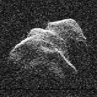
The image at the top of the page is of asteroid 2012 LZ1.
"On Sunday, June 10, a potentially hazardous asteroid thought to have been 500 meters (0.31 miles) wide was discovered by Siding Spring Observatory in New South Wales, Australia. Fortunately for us, asteroid 2012 LZ1 drifted safely by, coming within 14 lunar distances from Earth on Thursday, June 14."[28]
"Asteroid 2012 LZ1 is actually bigger than thought… in fact, it is quite a lot bigger. 2012 LZ1 is one kilometer wide (0.62 miles), double the initial estimate."[28]
Asteroid "2012 LZ1′s surface is really dark, reflecting only 2-4 percent of the light that hits it — this contributed to the underestimated initial optical observations. Looking for an asteroid the shade of charcoal isn’t easy."[28]
“This object turned out to be quite a bit bigger than we expected, which shows how important radar observations can be, because we’re still learning a lot about the population of asteroids”.[29]
“The sensitivity of our radar has permitted us to measure this asteroid’s properties and determine that it will not impact the Earth at least in the next 750 years”.[30]
The extremely accurate astrometry provided by radar is critical in long-term predictions of asteroid-Earth impacts, as illustrated by the object 99942 Apophis.
At right is a Goldstone radar image of the asteroid 4179 Toutatis on November 26, 1996.
The "images were recorded at NASA's Deep Space Network 70-meter and 34-meter radio/radar antennas in Goldstone, CA, and the 305-meter Arecibo Radio Telescope in Puerto Rico."[31]
"It's amazing that the shape of Toutatis can be determined so accurately from ground-based observations".[32]
"This technology will provide us with startling, close-up views of thousands of asteroids that orbit near the Earth."[32]
"We used the computer to mathematically create a three- dimensional model of the surface and rotation of Toutatis".[33]
"It's as though we put a clay model in space and molded it until it matched the appearance of the actual asteroid."[33]
"The video is of particular interest as Toutatis nears Earth and makes its closest approach on Friday, Nov. 29, when it will pass by at a distance of 3.3 million miles (5.3 million kilometers), or about 14 times the distance from the Earth to the Moon. In 2004, Toutatis will pass only four lunar distances from Earth, closer than any known Earth- approaching object expected to pass by in the next 60 years."[31]
"Toutatis poses no significant threat to Earth, at least for a few hundred years".[34]
"The discovery that we live in an asteroid swarm is important for the future of humanity".[34]
"These leftover debris from planetary formation can teach us a good deal about the formation of our Solar System. Asteroids also contain valuable minerals and many are the cheapest possible destinations for space missions."[34]
16 Psyche
[edit | edit source]
A "huge, metallic asteroid named 16 Psyche [...] resides" in the asteroid belt.[35]
16 Psyche is "a 130-mile-wide (210 kilometers) metallic asteroid that may be the core of an ancient, Mars-size planet. Violent collisions billions of years ago might have stripped away the layers of rock that once lay atop this metallic object."[36]
"16 Psyche is the only known object of its kind in the solar system, and this is the only way humans will ever visit a core. We learn about inner space by visiting outer space."[36]
The "asteroid Psyche displays significant variations in radar and optical albedo with rotation."[37]
"16 Psyche [is] the largest M-class asteroid in the main belt."[37]
"18 radar imaging and 6 continuous wave runs in November and December 2015, [were] combined [...] with 16 continuous wave runs from 2005 and 6 recent adaptive-optics (AO) images (Drummond et al., 2016) to generate a three-dimensional shape model of Psyche."[37]
The "shape model has dimensions 279 × 232 × 189 km (± 10%), Deff = 226 ± 23 km, and is 6% larger than, but within the uncertainties of, the most recently published size and shape model generated from the inversion of lightcurves (Hanus et al., 2013). Psyche is roughly ellipsoidal but displays a mass-deficit over a region spanning 90° of longitude. There is also evidence for two ∼50–70 km wide depressions near its south pole. Their size and published masses lead to an overall bulk density estimate of 4500 ± 1400 kg·m−3. Psyche's mean radar albedo of 0.37 ± 0.09 is consistent with a near-surface regolith composed largely of iron-nickel and ∼40% porosity. Its radar reflectivity varies by a factor of 1.6 as the asteroid rotates, suggesting global variations in metal abundance or bulk density in the near surface."[37]
Jupiter
[edit | edit source]
"Details in radiation belts close to Jupiter are mapped from measurements that NASA's Cassini spacecraft made of radio emission from high-energy electrons moving at nearly the speed of light within the belts."[38]
"The three views show the belts at different points in Jupiter's 10-hour rotation. A picture of Jupiter is superimposed to show the size of the belts relative to the planet. Cassini's radar instrument, operating in a listen-only mode, measured the strength of microwave radio emissions at a frequency of 13.8 gigahertz (13.8 billion cycles per second or 2.2 centimeter wavelength). The results indicate the region near Jupiter is one of the harshest radiation environments in the solar system."[38]
"From Earth-based radio telescopes, the telltale radio emissions would be swamped out by heat-generated radio emissions from Jupiter's atmosphere, but Cassini was close enough to Jupiter in January 2001 to differentiate between the emissions from the radiation belts and those from the atmosphere."[38]
"The belts appear to wobble as the planet turns because they are controlled by Jupiter's magnetic field, which is tilted in relation to the planet's poles."[38]
Between September and November 23, 1963, Jupiter is detected by radar astronomy.[39]
"The dense atmosphere makes a penetration to a hard surface (if indeed one exists at all) very unlikely. In fact, the JPL results imply a correlation of the echo with Jupiter ... which corresponds to the upper (visible) atmosphere. ... Further observations will be needed to clarify the current uncertainties surrounding radar observations of Jupiter."[39]
"Although in 1963 some claimed to have detected echoes from Jupiter, these were quite weak and have not been verified by later experiments."[40]
"A search for radar echoes from Jupiter at 430 MHz during the oppositions of 1964 and 1965 failed to yield positive results, despite a sensitivity several orders of magnitude better than employed by other groups in earlier (1963) attempts at higher frequencies. ... [I]t might be suspected that meteorological disturbances of a random nature were involved, and that the echoes might be returned only in exceptional circumstances. Further support for this point of view may be gleaned from the fact that JPL found positive results for only 1 (centered at 32° System I longitude) of the 8 longitude regions investigated in 1963 (Goldstein 1964) and, in fact, had no success during their observations in 1964 (see comment by Goldstein following Dyce 1965)."[41]
Titan
[edit | edit source]

Radar detection of Titan from Arecibo Observatory, included mapping of Titan's surface.
"This Cassini false-color mosaic [at right] shows all synthetic-aperture radar images to date of Titan's north polar region. Approximately 60 percent of Titan's north polar region, above 60 degrees north latitude, is now mapped with radar. About 14 percent of the mapped region is covered by what is interpreted as liquid hydrocarbon lakes."[42]
"Features thought to be liquid are shown in blue and black, and the areas likely to be solid surface are tinted brown. The terrain in the upper left of this mosaic is imaged at lower resolution than the remainder of the image".[42]
"Most of the many lakes and seas seen so far are contained in this image, including the largest known body of liquid on Titan. These seas are most likely filled with liquid ethane, methane and dissolved nitrogen."[42]
"Many bays, islands and presumed tributary networks are associated with the seas. The large feature in the upper right center of this image is at least 100,000 square kilometers (40,000 square miles) in area, greater in extent than Lake Superior (82,000 square kilometers or 32,000 square miles), one of Earth's largest lakes. This Titan feature covers a greater fraction of the surface, at least 0.12 percent, than the Black Sea, Earth's largest terrestrial inland sea, at 0.085 percent. Larger seas may exist, as it is probable that some of these bodies are connected, either in areas unmapped by radar or under the surface (see PIA08365)."[42]
"Of the 400 observed lakes and seas, 70 percent of their area is taken up by large "seas" greater than 26,000 square kilometers (10,000 square miles)."[42]
In the second image at right is another radar image of Titan's surface. "The existence of oceans or lakes of liquid methane on Saturn's moon Titan was predicted more than 20 years ago. But with a dense haze preventing a closer look it has not been possible to confirm their presence. Until the Cassini flyby of July 22, 2006, that is."[43]
"Radar imaging data from the flyby, published this week in the journal Nature, provide convincing evidence for large bodies of liquid. This image, used on the journal's cover, gives a taste of what Cassini saw. Intensity in this colorized image is proportional to how much radar brightness is returned, or more specifically, the logarithm of the radar backscatter cross-section. The colors are not a representation of what the human eye would see."[43]
"The lakes, darker than the surrounding terrain, are emphasized here by tinting regions of low backscatter in blue. Radar-brighter regions are shown in tan. The strip of radar imagery is foreshortened to simulate an oblique view of the highest latitude region, seen from a point to its west."[43]
"This radar image was acquired by the Cassini radar instrument in synthetic aperture mode on July 22, 2006. The image is centered near 80 degrees north, 35 degrees west and is about 140 kilometers (84 miles) across. Smallest details in this image are about 500 meters (1,640 feet) across."[43]
Comets
[edit | edit source]"Goldstone radar observations on 2011 August 19 and 20 detected echoes from the nucleus and coma of comet 45P/Honda-Mrkos-Pajdusakova (HMP). This is only the fourth Goldstone comet detection and the first since detection of comet 73P/Schwassmann-Wachmann 3 in 2006."[44]
"The [continuous wave] CW spectrum [on the right] shows the opposite-circular echo from the comet obtained on August 19. The narrow spike is the echo from the nucleus and the broad, low, asymmetric hump is the echo from coma particles. The skew of the coma echo to positive frequencies indicates that most of the coma particles were approaching Earth at the time of the observations."[44]
"The Goldstone measurements provided a range correction of 49 km for the nucleus, which significantly improved the orbit and which revealed a systematic bias in many of the optical observations."[44]
"This is only the fifteenth comet that has been detected with radar."[44]
Astrometry
[edit | edit source]
"Asteroid radar astronomy began on 14 June 1968, with the detection of 1566 Icarus from Goldstone (Goldstein 1969) and Haystack (Pettengill et al. 1969)."[45]
"Radar measurements of echo Doppler frequencies and time delays permit significant refinements of orbital elements and commensurate improvements in the accuracy of prediction ephemerides because these measurements have fine fractional precision and are orthogonal to optical, angular-position measurements."[45]
"Yeomans et al. (1987) used numerical experiments to explore the extent to which delay/ Doppler astrometry can refine orbit estimates for NEAs. They concluded that radar measurements can reduce ephemeris uncertainties dramatically for asteroids having short optical-data histories. They noted that a few radar observations of a newly discovered NEA could mean the difference between successfully recovering the object during its next close approach and losing it entirely. Even for asteroids with very long astrometric histories and secure orbits, radar measurements can significantly shrink their positional error ellipsoids for at least a decade."[45]
"A typical transmit/receive cycle, or run, consists of signal transmission for a duration close to the roundtrip light time between the radar and the target, i.e., until the first echoes are about to come back, followed by reception of echoes for a similar duration. In continuous wave (cw) observations, one transmits a nearly monochromatic waveform and measures the distribution of echo power as a function of frequency. The resultant echo spectra can be thought of as one-dimensional images, or brightness scans across the target through a slit parallel to the asteroid’s apparent spin vector. In ranging observations, time coding of the waveform permits measurement of the distribution of echo power in time delay (range) as well."[45]
"An asteroid’s apparent radial motion introduces a continuously changing Doppler shift into the echoes. One avoids spectral smear by tuning the receiver according to an ephemeris based on an orbit determined from astrometric asteroid observations."[45]
"In cw experiments, voltage samples of the received signal are Fourier transformed and the results are squared to obtain an estimate of the power spectrum, with the frequency resolution equal to the reciprocal of the time series length, i.e., of the coherence time. The sampling rate is chosen to provide an unaliased bandwidth many times larger than both the a priori Doppler uncertainty and the echo bandwidth, so fest can be determined unambiguously from the received power spectrum. Normally, a number of these "single-look" spectra are averaged to improve the spectral estimates."[45]
"In principle, range resolution can be obtained by using a coherent pulsed cw waveform—the transmitter’s carrier-frequency oscillator operates continuously but radio-frequency power is radiated only during intervals that are one delay resolution cell long and occur at intervals called the pulse repetition period (PRP). The PRP is normally much greater than the target’s intrinsic delay dispersion, thereby ensuring that the echo will consist of successive, nonoverlapping range profiles. Fourier transformation of N time samples taken at the same position (i.e., the same delay relative to τ0) within each of N successive range profiles yields the echo power spectrum for the corresponding range cell on the target. This spectrum has an unaliased bandwidth B - l/[(PRP)(NCOH)] and a frequency resolution B/N, where NCOH is the number of code cycles for which voltage samples have been coherently summed prior to Fourier transformation."[45]
Locations on Earth
[edit | edit source]

The radar image of France on the right is color-coded for relative relief from darker green at or near sea level to white for mountain tops. The border of France has been shaded and given a slight elevation away from the rest of the Earth nearby.
On the left is a colour coded TanDEM-X digital elevation model is of Khairabad in northern Pakistan, created on 6 August 2010.
Paleogeography
[edit | edit source]
"The ability of a sophisticated radar instrument to image large regions of the world from space, using different frequencies that can penetrate dry sand cover, produced the discovery in this image: a previously unknown branch of an ancient river, buried under thousands of years of windblown sand in a region of the Sahara Desert in North Africa. This area is near the Kufra Oasis in southeast Libya, centered at 23.3 degrees north latitude, 22.9 degrees east longitude. The image was acquired by the Spaceborne Imaging Radar-C/X-band Synthetic Aperture (SIR- C/X-SAR) imaging radar when it flew aboard the space shuttle Endeavour on its 60th orbit on October 4, 1994. This SIR-C image reveals a system of old, now inactive stream valleys, called "paleodrainage systems.""[46]
Impact craters
[edit | edit source]Per the image on the right: "In 2015 I was looking at a new map of the bedrock below the Greenland Ice Sheet and discovered a large circular feature under the Hiawatha glacier in northwest Greenland."[47]
"You can see the rounded structure at the edge of the ice sheet, especially when flying high enough."[48]
"For the most part the crater isn’t visible out the airplane window. It’s funny that until now nobody thought, ‘Hey, what’s that semicircular feature there?’ From the airplane it is subtle and hard to see unless you already know it’s there. Using satellite imagery taken at a low sun angle that accentuates hills and valleys in the ice sheet’s terrain—you can really see the circle of the whole crater in these images."[48]
"It is correct that the crater is not well dated but there’s good evidence that it is geologically young, that is, it formed within the last 2 to 3 million years, and most likely it is as young as the last Ice Age [which ended around 12,000 years ago],” Larsen explained to Gizmodo. “We are currently trying to come up with ideas on how to date the impact. One idea is to drill through the ice and get bedrock samples that can be used for numerical dating."[47]
On the left is an image of bed "topography based on airborne radar sounding from 1997 to 2014 NASA data and 2016 Alfred Wegener Institute (AWI) data. Black triangles represent elevated rim picks from the radargrams, and the dark purple circles represent peaks in the central uplift. Hatched red lines are field measurements of the strike of ice-marginal bedrock structures. Black circles show location of the three glaciofluvial sediment samples".[49]
"Glaciofluvial sediment from the largest river draining the crater contains shocked quartz and other impact-related grains. Geochemical analysis of this sediment indicates that the impactor was a fractionated iron asteroid, which must have been more than a kilometer wide to produce the identified crater. Radiostratigraphy of the ice in the crater shows that the Holocene ice is continuous and conformable, but all deeper and older ice appears to be debris rich or heavily disturbed."[49]
Rainbands
[edit | edit source]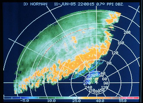
Rainbands are cloud and precipitation areas which are significantly elongated. Rainbands can be stratiform or convective,[50] and are generated by differences in temperature. When noted on weather radar imagery, this precipitation elongation is referred to as banded structure.[51] Rainbands in advance of warm occluded fronts and warm fronts are associated with weak upward motion,[52] and tend to be wide and stratiform in nature.[53]
Rainbands spawned near and ahead of cold fronts can be squall lines which are able to produce tornadoes.[54] Rainbands associated with cold fronts can be warped by mountain barriers perpendicular to the front's orientation due to the formation of a low-level barrier jet.[55] Bands of thunderstorms can form with sea breeze and land breeze boundaries, if enough moisture is present. If sea breeze rainbands become active enough just ahead of a cold front, they can mask the location of the cold front itself.[56]
Extratropical cyclones
[edit | edit source]
Rainbands in advance of warm occluded fronts and warm fronts are associated with weak upward motion,[57] and tend to be wide and stratiform in nature.[58] In an atmosphere with rich low level moisture and vertical wind shear,[59] narrow, convective rainbands known as squall lines generally in the cyclone's warm sector, ahead of strong cold fronts associated with extratropical cyclones.[60] Wider rain bands can occur behind cold fronts, which tend to have more stratiform, and less convective, precipitation.[61] Within the cold sector north to northwest of a cyclone center, in colder cyclones, small scale, or mesoscale, bands of heavy snow can occur within a cyclone's comma head precipitation pattern with a width of 32 kilometres (20 mi) to 80 kilometres (50 mi).[62] These bands in the comma head are associated with areas of frontogensis, or zones of strengthening temperature contrast.[63] Southwest of extratropical cyclones, curved flow bringing cold air across the relatively warm Great Lakes can lead to narrow lake effect snow bands which bring significant localized snowfall.[64]
Recent history
[edit | edit source]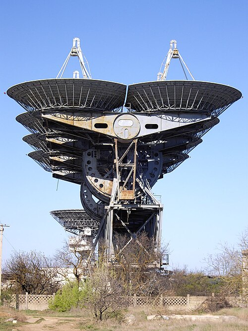
The recent history period dates from around 1,000 b2k to present.
The "Arecibo telescope was completed in 1963 at the initiative of Cornell electrical engineering professor William E. Gordon".[65]
At right is an image of the Pluton radar complex used for radar astronomy since 1960.
Arecibo Observatory
[edit | edit source]The "Arecibo Observatory in Puerto Rico [is] the world's largest, and most sensitive, single-dish radio telescope."[65]
"The 1,000-foot-diameter (305 meters) Arecibo telescope [... provides] access to state-of-the-art observing for scientists in radio astronomy, solar system radar and atmospheric studies, and the observatory has the unique capability for solar system and ionosphere (the atmosphere's ionized upper layers) radar remote sensing."[65] It contains the largest curved focusing dish on Earth, giving Arecibo the largest electromagnetic-wave-gathering capacity.[66] The dish surface is made of 38,778 perforated aluminum panels, each measuring about 3 by 6 feet (1 by 2 m), supported by a mesh of steel cables.
The telescope has three radar transmitters, with effective isotropic radiated powers [EIRP] of 20 TW at 2380 MHz, 2.5 TW (pulse peak) at 430 MHz, and 300 MW at 47 MHz. The telescope is a spherical reflector, not a parabolic reflector. To aim the telescope, the receiver is moved to intercept signals reflected from different directions by the spherical dish surface. A parabolic mirror would induce a varying astigmatism when the receiver is in different positions off the focal point, but the error of a spherical mirror is the same in every direction.
The receiver is located on a 900-ton platform which is suspended 150 m (500 ft) in the air above the dish by 18 cables running from three reinforced concrete towers, one of which is 110 m (365 ft) high and the other two of which are 80 m (265 ft) high (the tops of the three towers are at the same elevation). The platform has a 93-meter-long rotating bow-shaped track called the azimuth arm on which receiving antennas, secondary and tertiary reflectors are mounted. This allows the telescope to observe any region of the sky within a forty-degree cone of visibility about the local zenith (between −1 and 38 degrees of declination). Puerto Rico's location near the equator allows Arecibo to view all of the planets in the Solar System, though the round trip light time to objects beyond Saturn is longer than the time the telescope can track it, preventing radar observations of more distant objects.
Goldstone Deep Space Communication Complex
[edit | edit source]
Shown at right are the three "34m (110 ft.) diameter Beam Waveguide antennas located at the Goldstone Deep Space Communications Complex, situated in the Mojave Desert in California. This is one of three complexes which comprise NASA's Deep Space Network (DSN). The DSN provides radio communications for all of NASA's interplanetary spacecraft and is also utilized for radio astronomy and radar observations of the solar system and the universe."[67]
Shuttle radar imaging
[edit | edit source]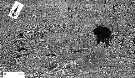


The Shuttle Imaging Radar-A (SIR-A) was for remote sensing of Earth's resources. Experiments were conducted by Shuttle missions: STS-2.
The Shuttle Imaging Radar-B (SIR-B) was part of the OSTA-3 experiment package (Spacelab) in the payload bay of STS-13.
The SIR-B was an improved version of a similar device flown on the OSTA-1 package during STS-2. It had an eight-panel antenna array measuring 11 × 2 m (36.1 × 6.6 ft). It operated throughout the flight, but much of the data had to be recorded on board the orbiter rather than transmitted to Earth in real-time as was originally planned.
SIR-B radar image of the Sudbury impact structure (elliptical because of deformation by Grenville thrusting) and the nearby Wanapitei crater (lake-filled) formed much later. The partially circular lake-filled structure on the right (east) is the 8 km (5 mi) wide Wanapitei crater, estimated to have formed 34 million years (m.y.) ago. The far larger Sudbury structure (second largest on Earth) appears as a pronounced elliptical pattern, more strongly expressed by the low hills to the north. This huge impact crater, with its distinctive outline, was created about 1800 m.y. ago. Some scientists argue that it was at least 245 km (152 mi) across when it was circular. More than 900 m.y. later strong northwestward thrusting of the Grenville Province terrane against the Superior Province (containing Sudbury) subsequently deformed it into its present elliptical shape (geologists will recognize this as a prime example of the "strain ellipsoid" model). After Sudbury was initially excavated, magmas from deep in the crust invaded the breccia filling, mixing with it and forming a boundary layer against its walls. Some investigators think that the resulting norite rocks are actually melted target rocks. This igneous rock (called an "irruptive") is host to vast deposits of nickel and copper, making this impact structure a 5 billion dollar source of ore minerals since mining began in the last century.
This radar image shows the Teide volcano on the island of Tenerife in the Canary Islands. The Canary Islands, part of Spain, are located in the eastern Atlantic Ocean off the coast of Morocco. Teide has erupted only once in the 20th Century, in 1909, but is considered a potentially threatening volcano due to its proximity to the city of Santa Cruz de Tenerife, shown in this image as the purple and white area on the lower right edge of the island. The summit crater of Teide, clearly visible in the left center of the image, contains lava flows of various ages and roughnesses that appear in shades of green and brown. Different vegetation zones, both natural and agricultural, are detected by the radar as areas of purple, green and yellow on the volcano's flanks. Scientists are using images such as this to understand the evolution of the structure of Teide, especially the formation of the summit caldera and the potential for collapse of the flanks. The volcano is one of 15 identified by scientists as potentially hazardous to local populations, as part of the international cooperation agreement.
The image was acquired by the Spaceborne Imaging Radar-C/X-Band Synthetic Aperture Radar (SIR-C/X-SAR) onboard the space shuttle Endeavour on October 11, 1994, Space Transportation System-65. SIR-C/X-SAR, a joint mission of the German, Italian and the United States space agencies, is part of NASA's Mission to Planet Earth. The image is centered at 28.3 degrees North latitude and 16.6 degrees West longitude. North is toward the upper right. The area shown measures 90 kilometers by 54.5 kilometers (55.8 miles by 33.8 miles). The colors in the image are assigned to different frequencies and polarizations of the radar as follows: red is L-band horizontally transmitted, horizontally received; green is L-band horizontally transmitted, vertically received; blue is C-band horizontally transmitted, vertically received.
STS-52: delivered (3) an Orbital Debris Radar Calibration System (ODERACS), an experiment which released 6 calibrated spheres into orbit in order to provide a source for fine-tuning ground-based radar facilities around the world.
Space Transportation System-65: The primary payload is the Space Radar Laboratory (SRL-2), making its second flight to study the Earth's environment.
On Friday, 30 September 1994 at 5 pm CDT, Space Transportation System-65 MCC Status Report # 2 reports: Shortly after 4 pm that day, flight controllers reported that the on-orbit checkout of the Spaceborne Imaging Radar-C (SIR-C) and the Synthetic Aperture Radar (X-SAR) had been completed, and that the primary SRL-2 instruments were ready for operation. Throughout the checkout, data takes were recorded over a number of sites, including Raco, Michigan; Bermuda; Bebedouro, Brazil; the Northeast Pacific Ocean and the Juan de Fuca Strait, between the United States and Canada.
On Saturday, 1 October 1994 at 9 am CDT, Space Transportation System-65 MCC Status Report # 3 reports: Environmental studies continued throughout Saturday morning aboard Endeavour as six astronauts working around the clock in two shifts to assist the Space Radar Laboratory science team on the ground with real-time observations from space.
Commander Mike Baker and Pilot Terry Wilcutt made attitude adjustments of the orbiter to assist in precisely pointing the radar systems.
The SRL team performed a series of data takes using the radar equipment as Endeavour moved over that area of the world. Those images will be compared with similar radar images gathered during the Space Transportation System-62 (STS-59) mission in April, prior to the volcanic activity. Other radar data gathering of the Earth's surface today included the desert regions of Africa, both the Pacific and Atlantic Oceans and mountainous regions of the East and West coasts of the United States.
On Sunday, 2 October 1994 at 9 am CDT, Space Transportation System-65 MCC Status Report # 4 reports: Radar data gathering today included forest areas of North Carolina, ocean current patterns in the Atlantic and Pacific Oceans, desert areas in Africa, and mountainous regions of the East and West coasts of the United States.
On Monday, 3 October 1994 at 10 am CDT, STS-68 MCC Status Report # 5 reports: Endeavour's Space Radar Laboratory equipment continued to search the Earth's land masses and oceans for environmental changes that have occurred since the last SRL mission in April.
The Red Team of Mike Baker, Terry Wilcutt and Jeff Wisoff were on duty throughout much of the day. Radar data gathered today included much of the East Coast of the United States, current patterns in the Atlantic and Pacific Oceans as well as other bodies of water, desert areas in Africa, and mountainous regions around the world.
On Monday, 3 October 1994 at 5 pm CDT, Space Transportation System-65 MCC Status Report # 6 reports: Endeavour's payload bay cameras sent to Earth dramatic video of the western coast of Oregon and the length of California and the Baja Peninsula that scientists will compare with radar images downlinked from Space Radar Laboratory-2 instruments earlier in the flight. The observations were part of a continuing effort to watch the Earth below for evidence of environmental changes that have occurred since the last SRL mission in April. The overall goal of the mission to better understand the differences in changes caused by natural processes and compare them to changes brought about by human activity. Radar data was recorded today over much of the East Coast of the United States, the Atlantic and Pacific Oceans, Manitoba, Canada, and French Guiana.
Astronauts relayed information about storms, lightning, fires and clear cutting to the SRL science team that will be used to help understand the radar images and MAPS data on carbon monoxide levels in the atmosphere.
On Tuesday, 4 October 1994 at 9 am CDT, Space Transportation System-65 (STS-68) MCC Status Report # 7 reports: STS-68 crew members this morning performed two slight maneuvers to fine-tune Endeavour's orbit to mirror its track on the first Space Radar Laboratory mission to support a new experiment called interferometry. The trim burns adjust the orbit to within 10 metres (33 ft) of where it was in April which will allow scientists to make near identical measurements with the radar equipment to develop a three-dimensional comparison of environmental changes during the six months separating the two missions—Space Transportation System-62 (STS-59) and STS-68.
On Tuesday, 4 October 1994 at 5 pm CDT, Space Transportation System-65 (STS-68) MCC Status Report # 8 reports: Space Radar Laboratory-2 scientists adjusted their observation plans to take advantage of an opportunity to train their instruments on the islands of Japan following a Tuesday night earthquake there. Endeavour passed over the Sarobetsu, Japan, calibration site about 3:30 pm CDT, and the Synthetic Aperture Radar sent down real-time data of the area below, allowing scientists to look for changes in the coastline of the islands that may have been due to the large tsunami waves associated with the quake. The Spaceborne Imaging Radar also recorded data on the area.
STS-68 crew members continued to perform slight maneuvers to fine-tune Endeavour's orbit to intersect its track on the SRL-1 mission to support a new experiment called interferometry. The trim burns adjusted the orbit to within 30 feet (9.1 m) of where it was in April as it passed over the Mammoth Mountain, Calif., backup supersite. This should allow scientists to make nearly identical measurements with the radar equipment to develop a three-dimensional comparison of environmental changes during the six months separating Space Transportation System-62 (STS-59) and Space Transportation System-65 (STS-68).
Radar images over the Sahara desert and the North Atlantic will help scientists evaluate global changes and how they affect the climates in other areas of the world.
Also on 4 October, Payload Commander Tom Jones discussed the significance of radar systems and the Earth's environment in an interview with ABC's Good Morning America. Mission Specialist Jeff Wisoff discussed the mission with CONUS Communications Syndicate affiliates WTKR-TV in his hometown of Norfolk, Va., and the All-News Channel in Minneapolis.
On Wednesday, 5 October 1994 at 8 am CDT, Space Transportation System-65 (STS-68) MCC Status Report # 9 reports: Space Radar Laboratory scientists received some images of Japan, near the location of Monday nights earthquake, but any evidence of the natural disaster was not immediately noticeable. Other radar observations during the night included studies of other volcanoes including Mt. Pinatubo in the Philippines, Cotopaxi in Ecuador, and Teide in the Canary Islands.
Radar images processed on the ground included images of Pasadena, California, with sufficient clarity make the Rose Bowl distinguishable, as well as images of Washington State and Yellowstone National Park, both showing scars from forest fires.
During the night, the crew reported a missing thermal tile around one of the overhead windows of the orbiter. The tile apparently came off recently since crew members look out the window often to perform the visual observations that accompany radar operations. Flight controllers report that, while the tile is missing, the underlying thermal blanket is still intact.
Astronaut Linda Godwin, who served as the payload commander on the first Space Radar Laboratory mission in April, briefed the crew from the payload control room about 4:30 am Wednesday, commemorating the tenth anniversary of Challenger's 41-G mission, which carried the Spaceborne Imaging Radar (SIR-B) and the Measurement of Air Pollution by Satellite (MAPS). She also noted the first flight aboard a Shuttle of that radar-imaging equipment on Columbia in November 1981.
On Wednesday, 5 October 1994 at 4 pm CDT, Space Transportation System-65 (STS-68) MCC Status Report # 10 reports: Mission to Planet Earth observations by Endeavour's payload bay radar instruments were being suspended temporarily Wednesday afternoon to save fuel while flight controllers work to fix a minor problem involving the shuttle's small reaction control system jets.
The radar instruments earlier Wednesday collected images over the Kliuchevskoi volcano in Kamchatka, Russia, which erupted about 8 hours after Endeavour's launch Friday. Images also were collected over Yellowstone National Park, Wyo.; Chickasha, Okla.; Ruiz, Columbia; Cuprito, Nevada; Colima, Mexico; the Galapagos Islands and San Juan, Argentina. Observations with the Measurement of Air Pollution from Satellite were taken, with one particular target being line fires in British Columbia, Canada.
On Thursday, 6 October 1994 at 8 am CDT, Space Transportation System-65 (STS-68) MCC Status Report # 11 reports: Endeavour's small steering jets are now back in continuous operation and Space Radar Laboratory observations are continuing on schedule after Mission Control sent a software update to the shuttle about 3:30 am today.
The software patch accommodated a failed temperature sensor in one of the vernier jets and allows Endeavour's onboard computers to track the operation of the jet via a second sensor located near the failed sensor. While the patch was being developed and tested in simulators, observations by the Space Radar Laboratory continued at a reduced pace.
The observations using the radar systems that were missed while the software patch was being put in place, had been performed at least once previously during the mission and are scheduled for observation again later in the flight. SRL scientists say the impact of the temporary pause is minimal on the scientific investigations under way.
One observation completed during the night was of a controlled oil spill in the North Sea designed to test the radar's ability to discern oil spills from the naturally produced film caused by fish and plankton in the water. In addition to the 106 gallons of diesel oil placed in the water, 26 gallons of algae products were placed in the water nearby for radar comparison. The ground team expected to have the oil spill cleaned up within about two hours using oil-recovery ships in the area. The experiment was conducted to prove the usefulness of radar systems to more rapidly detect spills allowing quicker cleanup.
On Thursday, 6 October 1994 at 5 pm CDT, Space Transportation System-65 (STS-68) MCC Status Report # 12 reports: Endeavour's astronauts this afternoon sent down spectacular videotape views of the west coast of California recorded as the shuttle passed about 115 nautical miles (213 km) overhead on its 103rd orbit. The scenes covered the San Joaquin Valley, San Francisco Bay, Monterey Bay, Los Angeles, Vandenberg Air Force Base and San Diego Bay. During the next few days, scientists will test a new technique called "interferometry" as the earth observations data collection continues. The technique is expected to yield topographic information of unprecedented clarity by using slightly different shuttle positions to provide three-dimensional images of the terrain below. Among the Space Radar Laboratory observations today were the North Sea, where scientists intentionally released small oil and algae spills to see how well the SRL-2 instruments could track them, as well as observations of Bebedouro, Brazil; the Western and Northeast Pacific Ocean; Chickasha, Oklahoma; the Gulf of Mexico; Ruiz, Colombia; Sena Madureira, Brazil; Weddell Sea; the Kliuchevskoi Volcano in Kamchatmka; Stovepipe Wells, California; and the Galapagos Islands. Earlier today, the Mission Management Team extended STS-68 by one day to allow additional science. Endeavour is now expected to land at the Kennedy Space Center at about 10:36 am Tuesday.
On Friday, 7 October 1994 at 8 am CDT, Space Transportation System-65 (STS-68) MCC Status Report # 13 reports: Observations made during the night included the volcano Merapi on the Indonesian island of Java; Duke Forest in North Carolina; the Gulf of St. Lawrence; Sydney, Australia; and the volcano Mt. Pinatubo in the Philippines. Tom Jones, the Payload Commander for this second flight of SRL, spent some time this morning explaining the importance of the radar's volcanic studies. Demonstrating with three common types of volcanic rock, Jones explained how the radar's various frequencies allow it to map lava and ash flows around volcanoes. The work one day may lead to a permanent radar platform in orbit for use in assisting predictions of impending volcanic eruptions and safeguarding people living near active volcanoes. Late Thursday, Endeavour's astronauts sent down spectacular views of the west coast of California recorded as the shuttle passed about 115 nautical miles (213 km) overhead on its 103rd orbit. The scenes included the San Joaquin Valley, San Francisco, Monterey Bay, Los Angeles, Vandenberg Air Force Base and San Diego. On Friday, 7 October 1994 at 5 pm CDT, STS-68 MCC Status Report # 14 reports: Astronauts aboard Endeavour and Space Radar Laboratory-2 scientists on the ground today began in earnest to test the new technique of "interferometry" to produce even richer images of the Earth's surface.
From an altitude of 111 nautical miles (206 km), the Spaceborne Imaging Radar and Synthetic Aperture Radar recorded long swaths of interferometric data over central North America, the Amazon forests of central Brazil, and the volcanoes of the Kamchatka Peninsula in Russia.
The radar array aboard the shuttle began a series of observations above volcanoes, glaciers and other sites designed to create 3-D images. These spaceborne radar images, produced regularly on a long-term basis, eventually could provide scientists with insight into movements of the Earth's surface as small as a fraction of an inch.
Such close monitoring may allow scientists to detect pre-eruptive changes in volcanoes and movements in fault lines that precede earthquakes, providing an early warning of imminent natural hazards. Other future applications could include tracking the rate of global warming by monitoring the movement of glaciers and the tracking of floods and mudslides.
On Sunday, 9 October 1994 at 9 am CDT, Space Transportation System-65 (STS-68) MCC Status Report # 16 reports: It has seemed like deja vu on board Endeavour as the crew spent much of the last 24 hours precisely repeating many Space Radar Laboratory observations to provide scientists with duplicate images for highly accurate three-dimensional maps of volcanoes, glaciers and other phenomena.
Overnight, Mission Specialists Jeff Wisoff and Steve Smith replaced one of three payload recorders which malfunctioned yesterday. The procedure, which the two astronauts trained for prior to the mission, was completed in about an hour and a half. Although only two of the payload high data rate recorders were functioning, the planned observations by the radar lab were not interrupted. The two recorders alone were sufficient for retaining the radar data obtained during the overnight shift of astronauts Smith, Dan Bursch and Tom Jones.
Small engine firings by Endeavour late yesterday aligned the spacecraft's trajectory to within an estimated 20 metres (66 ft) of what had been planned when the spacecraft's orbit was lowered on Friday. This permits the precise repeat observations by the radar.
Interferometry data gathering with the radar instruments in the orbiter's payload bay continued throughout the night and morning prior to the scheduled deactivation of the X- band Synthetic Aperture Radar. Interferometry will allow scientists to overlay radar images of the same site taken on successive days forming a three-dimensional image of the Earth's surface. These topographical images can be used to create a baseline used to understand the changes in the environmental and ecological climate around the world.
Synthetic Aperture Radar Satellite
[edit | edit source]
"Using advanced radar imaging that will provide an unprecedented, detailed view of Earth, the NASA-ISRO Synthetic Aperture Radar, or NISAR, satellite is designed to observe and take measurements of some of the planet's most complex processes, including ecosystem disturbances, ice-sheet collapse, and natural hazards such as earthquakes, tsunamis, volcanoes and landslides."[68]
"Data collected from NISAR will reveal information about the evolution and state of Earth's crust, help scientists better understand our planet's processes and changing climate, and aid future resource and hazard management. The mission is a partnership between NASA and the Indian Space Research Organization [ISRO]."[68]
"Scientific Instrument(s) - L-band (24-centimeter wavelength) Polarimetric Synthetic Aperture Radar [JPL] - S-band (12-centimeter wavelength) Polarimetric Synthetic Aperture Radar [ISRO]"[68]
Interferograms
[edit | edit source]

"This image is an interferogram that was created using pairs of images taken by Synthetic Aperture Radar (SAR). The images, acquired at two different times, have been combined to measure surface deformation or changes that may have occurred during the time between data acquisition. The images were collected by the European Space Agency's Remote Sensing satellite (ERS-2) on 13 August 1999 and 17 September 1999 and were combined to produce these image maps of the apparent surface deformation, or changes, during and after the 17 August 1999 Izmit, Turkey earthquake. This magnitude 7.6 earthquake was the largest in 60 years in Turkey and caused extensive damage and loss of life. Each of the color contours of the interferogram represents 28 mm (1.1 inches) of motion towards the satellite, or about 70 mm (2.8 inches) of horizontal motion. White areas are outside the SAR image or water of seas and lakes. The North Anatolian Fault that broke during the Izmit earthquake moved more than 2.5 meters (8.1 feet) to produce the pattern measured by the interferogram. Thin red lines show the locations of fault breaks mapped on the surface. The SAR interferogram shows that the deformation and fault slip extended west of the surface faults, underneath the Gulf of Izmit. Thick black lines mark the fault rupture inferred from the SAR data. Scientists are using the SAR interferometry along with other data collected on the ground to estimate the pattern of slip that occurred during the Izmit earthquake. This then used to improve computer models that predict how this deformation transferred stress to other faults and to the continuation of the North Anatolian Fault, which extends to the west past the large city of Istanbul. These models show that the Izmit earthquake further increased the already high probability of a major earthquake near Istanbul."[69]
"This image [on the left] of Fort Irwin in California's Mojave Desert compares interferometric radar signatures topography -- data that were obtained by multiple imaging of the same region to produce three-dimensional elevation maps -- as it was obtained on October 7-8, 1994 by the Spaceborne Imaging Radar-C/X-band Synthetic Aperture Radar aboard the space shuttle Endeavour. Data were acquired using the L-band (24 centimeter wavelength) and C-band (6 centimeter wavelength). The image covers an area about 25 kilometers by 70 kilometers (15.5 miles by 43 miles). North is to the lower right of the image. The color contours shown are proportional to the topographic elevation. With a wavelength one-fourth that of the L-band, the results from the C-band cycle through the color contours four times faster for a given elevation change. Detailed comparisons of these multiple frequency data over different terrain types will provide insights in the future into wavelength-dependent effects of penetration and scattering on the topography measurement accuracy. Fort Irwin is an ideal site for such detailed digital elevation model comparisons because a number of high precision digital models of the area already exist from conventional measurements as well as from airborne interferometric SAR data."[70]
"Spaceborne Imaging Radar-C and X-band Synthetic Aperture Radar (SIR-C/X-SAR) is part of NASA's Mission to Planet Earth. The radars illuminate Earth with microwaves, allowing detailed observations at any time, regardless of weather or sunlight conditions. SIR-C/X-SAR uses three microwave wavelengths: L-band (24 cm), C-band (6 cm) and X-band (3 cm). The multi-frequency data will be used by the international scientific community to better understand the global environment and how it is changing. The SIR-C/X-SAR data, complemented by aircraft and ground studies, will give scientists clearer insights into those environmental changes which are caused by nature and those changes which are induced by human activity."[70]
"SIR-C was developed by NASA's Jet Propulsion Laboratory. X-SAR was developed by the Dornier and Alenia Spazio companies for the German space agency, Deutsche Agentur fuer Raumfahrtangelegenheiten (DARA), and the Italian space agency, Agenzia Spaziale Italiana (ASI), with the Deutsche Forschungsanstalt fuer Luft und Raumfahrt e.V.(DLR), the major partner in science, operations and data processing of X-SAR."[70]
Gyrotrons
[edit | edit source]
"Other important applications of gyrotrons are high-power microwave sources include high resolution radar ranging and imaging in atmospheric and planetary science as well as deep-space and specialized satellite communications and RF drivers for next-generation high-gradient linear accelerators".[71]
Aerial gravity gradiometry
[edit | edit source]The aircraft imaged on the right carried-out aerial high-resolution gravity gradiometry system in combination with LIDAR digital terrain mapping, electromagnetics, digital video, and gamma-ray spectrometry over "onshore areas along the South-Eastern Tanzanian Coastal Basin and the eastern arm of the East African Rift."[72]
Hypotheses
[edit | edit source]- A radar frequency exists that is reflected back by the Sun.
- A control group for radar astronomy would likely contain a standard target that allows maximum radar facility resolution and imaging.
See also
[edit | edit source]References
[edit | edit source]- ↑ J.S. Hey (1973). The Evolution of Radio Astronomy. Histories of Science Series. 1. Paul Elek (Scientific Books).
- ↑ 2.0 2.1 2.2 John W. Holt, Ali Safaeinili, Jeffrey J. Plaut, James W. Head, Roger J. Phillips, Roberto Seu, Scott D. Kempf, Prateek Choudhary, Duncan A. Young, Nathaniel E. Putzig, Daniela Biccari, Yonggyu Gim (November 2008). "Radar Sounding Evidence for Buried Glaciers in the Southern Mid-Latitudes of Mars". Science 322 (5905): 1235-8. doi:10.1126/science.1164246. http://www.sciencemag.org/content/322/5905/1235.full. Retrieved 2014-09-28.
- ↑ DLR (20 January 2011). The iceberg breaks free. Cologne: Deutsches Zentrum für Luft- und Raumfahrt. http://www.dlr.de/media/en/desktopdefault.aspx/tabid-4986/8423_read-18675/8423_page-2. Retrieved 2016-09-20.
- ↑ oldteched (December 1964). File:"Quill" satellite radar image of flooded Eel River outflow current.JPG. U. S. National Reconnaissance Office. https://commons.wikimedia.org/wiki/File:%22Quill%22_satellite_radar_image_of_flooded_Eel_River_outflow_current.JPG. Retrieved 2016-09-20.
- ↑ 5.0 5.1 5.2 5.3 Sue Lavoie (17 October 2001). PIA03458: Lost Hills, California Interferogram. Pasadena, California USA: NASA/JPL. http://photojournal.jpl.nasa.gov/catalog/PIA03458. Retrieved 2016-09-27.
- ↑ 6.0 6.1 6.2 6.3 6.4 Sue Lavoie (23 December 2002). PIA03376: Perspective View, SRTM / Landsat, Los Angeles, Calif. Pasadena, California USA: NASA/JPL. http://photojournal.jpl.nasa.gov/catalog/PIA03376. Retrieved 2016-09-27.
- ↑ 7.0 7.1 7.2 7.3 7.4 NASA/JPL/NGA (6 January 2005). PIA06661: Alpine Fault, New Zealand, SRTM Shaded Relief and Colored Height. Pasadena, California USA: NASA/JPL/NGA. http://photojournal.jpl.nasa.gov/catalog/PIA06661. Retrieved 2014-12-02.
- ↑ 8.0 8.1 8.2 8.3 8.4 Sue Lavoie (February 2000). "PIA06675: Ambae Island, Vanuatu (South Pacific)". Pasadena, California USA: NASA/JPL. Retrieved 2016-09-20.
- ↑ Annie Richardson and Al Wong (5 October 1994). "Photograph Identification: P-44823". Pasadena, California USA: NASA/JPL. Retrieved 2016-09-27.
- ↑ 10.0 10.1 Brian Dunbar (November 29, 2012). MESSENGER Finds New Evidence for Water Ice at Mercury's Poles. Washington, DC USA: NASA. http://www.nasa.gov/mission_pages/messenger/media/PressConf20121129.html. Retrieved 2013-10-24.
- ↑ 11.0 11.1 David Lawrence (November 29, 2012). MESSENGER Finds New Evidence for Water Ice at Mercury's Poles. Washington, DC USA: NASA. http://www.nasa.gov/mission_pages/messenger/media/PressConf20121129.html. Retrieved 2013-10-24.
- ↑ 12.0 12.1 Gregory Neumann (November 29, 2012). MESSENGER Finds New Evidence for Water Ice at Mercury's Poles. Washington, DC USA: NASA. http://www.nasa.gov/mission_pages/messenger/media/PressConf20121129.html. Retrieved 2013-10-24.
- ↑ David Paige (November 29, 2012). MESSENGER Finds New Evidence for Water Ice at Mercury's Poles. Washington, DC USA: NASA. http://www.nasa.gov/mission_pages/messenger/media/PressConf20121129.html. Retrieved 2013-10-24.
- ↑ M. A. Slade, B. J. Butler, D. O. Muhleman (1992). "Mercury radar imaging – Evidence for polar ice". Science 258 (5082): 635–640. doi:10.1126/science.258.5082.635. PMID 17748898.
- ↑ David R. Williams (June 2, 2005). Ice on Mercury. NASA Goddard Space Flight Center. http://nssdc.gsfc.nasa.gov/planetary/ice/ice_mercury.html. Retrieved 2008-05-23.
- ↑ Steven J. Ostro (October-December 1993). "Planetary radar astronomy". Reviews of Modern Physics 65 (4): 1235-79. doi:10.1103/RevModPhys.65.1235. http://rmp.aps.org/abstract/RMP/v65/i4/p1235_1. Retrieved 2012-02-09.
- ↑ 17.0 17.1 Al Wong (20 March 1996). Aorounga Impact Crater, Chad. Pasadena, California, USA: NASA/JPL. http://southport.jpl.nasa.gov/cdrom/sirced03/cdrom/DATA/LOCATION/AFRICA/SAHARA/POSTSIRC/CHAD.HTM. Retrieved 2016-09-15.
- ↑ J. Mofensen (February, April 1946). "Radar Echoes from the Moon". Nature, Electronics 157, 19 (3379): 129, 92-8. doi:10.1038/157129b0.
- ↑ Z. Bay, "Reflection of microwaves from the moon," Hung. Acta Phys., vol. 1, pp. 1-22; April, 1946.
- ↑ 20.0 20.1 20.2 20.3 20.4 P. Spudis (November 6, 2006). Ice on the Moon. The Space Review. http://www.thespacereview.com/article/740/1. Retrieved 12 April 2007.
- ↑ 21.0 21.1 Tony Greicius (December 6, 2012). "GRAIL's Gravity Map of the Moon". NASA/JPL-Caltech/MIT/GSFC. Retrieved 2012-12-15.
- ↑ 22.0 22.1 22.2 22.3 22.4 22.5 PR Newswire (December 5, 2012). NASA Twin Spacecraft Create Most Accurate Gravity Map Of Moon. http://news.yahoo.com/nasa-twin-spacecraft-create-most-accurate-gravity-map-173600085.html. Retrieved 2012-12-15.
- ↑ 23.0 23.1 23.2 S.G. Djorgovski. A Tour of the Radio Universe. National Radio Astronomy Observatory. http://www.cv.nrao.edu/course/astr534/Tour.html. Retrieved 2014-03-16.
- ↑ B. Gardini (2011). "ESA strategy for human exploration and the Lunar Lander Mission". Memorie della Societa Astronomica Italiana 82: 422-29. http://adsabs.harvard.edu/full/2011MmSAI..82..422G. Retrieved 5 May 2019.
- ↑ BatteryIncluded (June 14, 2013). File:PIA13164 North Polar Cap Cross Section, Annotated Version.jpg. San Francisco, California: Wikimedia Foundation, Inc. https://commons.wikimedia.org/wiki/File:PIA13164_North_Polar_Cap_Cross_Section,_Annotated_Version.jpg. Retrieved 2013-10-24.
- ↑ 26.0 26.1 26.2 Thomas Thompson (September 2, 2013). Radar Ionogram with Oblique Ionospheric Echo. Pasadena, California USA: NASA. http://mars.jpl.nasa.gov/express/gallery/martianterrain/MARSIS_release_4.html. Retrieved 2013-10-24.
- ↑ 27.0 27.1 27.2 27.3 27.4 27.5 27.6 Sue Lavoie (December 13, 2006). PIA09076: Interpreting Radar View near Mars' South Pole, Orbit 1334. Pasadena, California USA: NASA. http://photojournal.jpl.nasa.gov/catalog/PIA09076. Retrieved 2013-10-24.
- ↑ 28.0 28.1 28.2 Ian O'Neill (June 22, 2012). Asteroid 2012 LZ1 Just Got Supersized. Discovery Communications, LLC. http://news.discovery.com/space/asteroid-2012-lz1-just-got-supersized-120622.htm. Retrieved 2013-10-24.
- ↑ Ellen Howell (June 22, 2012). Asteroid 2012 LZ1 Just Got Supersized. Discovery Communications, LLC. http://news.discovery.com/space/asteroid-2012-lz1-just-got-supersized-120622.htm. Retrieved 2013-10-24.
- ↑ Mike Nolan (June 22, 2012). Asteroid 2012 LZ1 Just Got Supersized. Discovery Communications, LLC. http://news.discovery.com/space/asteroid-2012-lz1-just-got-supersized-120622.htm. Retrieved 2013-10-24.
- ↑ 31.0 31.1 Don Savage and Jane Platt (November 27, 1996). Images of Asteroid 4179 Toutatis. Washington, DC USA: NASA. http://neo.jpl.nasa.gov/images/toutatis.html. Retrieved 2013-10-24.
- ↑ 32.0 32.1 Eric De Jong (November 27, 1996). Images of Asteroid 4179 Toutatis. Washington, DC USA: NASA. http://neo.jpl.nasa.gov/images/toutatis.html. Retrieved 2013-10-24.
- ↑ 33.0 33.1 Scott Hudson (November 27, 1996). Images of Asteroid 4179 Toutatis. Washington, DC USA: NASA. http://neo.jpl.nasa.gov/images/toutatis.html. Retrieved 2013-10-24.
- ↑ 34.0 34.1 34.2 Steven Ostro (November 27, 1996). Images of Asteroid 4179 Toutatis. Washington, DC USA: NASA. http://neo.jpl.nasa.gov/images/toutatis.html. Retrieved 2013-10-24.
- ↑ Mike Wall (4 January 2017). NASA Unveils 2 New Missions to Study Truly Strange Asteroids. Space.com. http://www.space.com/35221-nasa-discovery-missions-asteroids-psyche-lucy.html. Retrieved 2017-01-09.
- ↑ 36.0 36.1 Lindy Elkins-Tanton (4 January 2017). NASA Unveils 2 New Missions to Study Truly Strange Asteroids. Space.com. http://www.space.com/35221-nasa-discovery-missions-asteroids-psyche-lucy.html. Retrieved 2017-01-09.
- ↑ 37.0 37.1 37.2 37.3 Imke de Pater (27 October 2016). Prof. Imke de Pater Confirms Asteroid 16 Psyche to be the Largest Metal Asteroid in the Main Belt. http://eps.berkeley.edu/news/prof-imke-de-pater-confirms-asteroid-16-psyche-be-largest-metal-asteroid-main-belt. Retrieved 2017-01-09.
- ↑ 38.0 38.1 38.2 38.3 Jim Wilson (27 February 2002). Inner Radiation Belts of Jupiter. Washington, DC USA: NASA. http://www.nasa.gov/mission_pages/juno/multimedia/pia03478.html. Retrieved 2016-11-06.
- ↑ 39.0 39.1 Gordon H. Pettengill & Irwin I. Shapiro (1965). "Radar Astronomy". Annual Review of Astronomy and Astrophysics 3: 377-410. http://adsabs.harvard.edu//abs/1965ARA&A...3..377P. Retrieved 2012-12-25.
- ↑ Irwin I. Shapiro (March 1968). "Planetary radar astronomy". Spectrum, IEEE 5 (3): 70-9. doi:10.1109/MSPEC.1968.5214821. http://ieeexplore.ieee.org/xpls/abs_all.jsp?arnumber=5214821. Retrieved 2012-12-25.
- ↑ R. B. Dyce and G. H. Pettengill, and A. D. Sanchez (August 1967). "Radar Observations of Mars and Jupiter at 70 cm". The Astronomical Journal 72 (4): 771-7. doi:10.1086/110307. http://articles.adsabs.harvard.edu/cgi-bin/nph-iarticle_query?1967AJ.....72..771D&data_type=PDF_HIGH&whole_paper=YES&type=PRINTER&filetype=.pdf. Retrieved 2012-12-25.
- ↑ 42.0 42.1 42.2 42.3 42.4 Sue Lavoie (October 11, 2007). PIA10008: Titan's North Polar Region. Pasadena, California USA: NASA/JPL. http://photojournal.jpl.nasa.gov/catalog/?IDNumber=PIA10008. Retrieved 2013-06-13.
- ↑ 43.0 43.1 43.2 43.3 Enrico Piazza (January 3, 2007). Liquid Lakes on Titan. Pasadena, California USA: NASA/JPL. http://saturn.jpl.nasa.gov/photos/imagedetails/index.cfm?imageId=2432. Retrieved 2013-06-13.
- ↑ 44.0 44.1 44.2 44.3 Goldstone (19 August 2011). GOLDSTONE RADAR DETECTION OF COMET HONDA-MRKOS-PAJDUSAKOVA. Pasasena, California USA: NASA/JPL. http://echo.jpl.nasa.gov/asteroids/45P_HMP/comet.hmp.html. Retrieved 2016-09-15.
- ↑ 45.0 45.1 45.2 45.3 45.4 45.5 45.6 Ostro, S. J.; Campbell, D. B.; Chandler, J. F.; Shapiro, I. I.; Hine, A. A.; Velez, R.; Jurgens, R. F.; Rosema, K. D.; Winkler, R.; Yeomans, D. K. (October 1991). "Asteroid radar astrometry". Astronomical Journal 102 (10): 1490-1502. doi:10.1086/115975. http://adsabs.harvard.edu/cgi-bin/nph-data_query?bibcode=1991AJ....102.1490O&link_type=ARTICLE&db_key=AST&high=. Retrieved 2017-07-27.
- ↑ Porao (4 October 1994). File:Kufra-space-radar.jpg. San Francisco, California: Wikimedia Foundation, Inc. https://commons.wikimedia.org/wiki/File:Kufra-space-radar.jpg. Retrieved 2016-09-27.
- ↑ 47.0 47.1 Nicolaj K. Larsen (14 November 2018). A Massive Impact Crater Has Been Detected Beneath Greenland’s Ice Sheet. Gizmodo. https://gizmodo.com/a-massive-impact-crater-has-been-detected-beneath-green-1830437095. Retrieved 14 November 2018.
- ↑ 48.0 48.1 John Paden (14 November 2018). A Massive Impact Crater Has Been Detected Beneath Greenland’s Ice Sheet. Gizmodo. https://gizmodo.com/a-massive-impact-crater-has-been-detected-beneath-green-1830437095. Retrieved 14 November 2018.
- ↑ 49.0 49.1 Kurt H. Kjær, Nicolaj K. Larsen, Tobias Binder, Anders A. Bjørk, Olaf Eisen, Mark A. Fahnestock, Svend Funder, Adam A. Garde, Henning Haack, Veit Helm, Michael Houmark-Nielsen, Kristian K. Kjeldsen1, Shfaqat A. Khan, Horst Machguth, Iain McDonald, Mathieu Morlighem, Jérémie Mouginot, John D. Paden, Tod E. Waight, Christian Weikusat, Eske Willerslev and Joseph A. MacGregor (14 November 2018). "A large impact crater beneath Hiawatha Glacier in northwest Greenland". Sciences Advances 4 (11): eaar8173. doi:10.1126/sciadv.aar8173. http://advances.sciencemag.org/content/4/11/eaar8173. Retrieved 14 November 2018.
- ↑ Glossary of Meteorology (2009). Rainband. [1] 2011-06-06 Retrieved on 2008-12-24.
- ↑ Glossary of Meteorology (2009). Banded structure. [2] 2011-06-06 Retrieved on 2008-12-24.
- ↑ Owen Hertzman (1988). Three-Dimensional Kinematics of Rainbands in Midlatitude Cyclones. Retrieved on 2008-12-24
- ↑ Yuh-Lang Lin (2007). Mesoscale Dynamics. Cambridge University Press. p. 405. ISBN 978-0-521-80875-0. https://books.google.com/books?id=4KXtnQ3bDeEC&pg=PA405.
- ↑ Glossary of Meteorology (2009). Prefrontal squall line. [url=https://web.archive.org/web/20070817224959/http://amsglossary.allenpress.com/glossary/search?id=prefrontal-squall-line1] 2007-08-17 Retrieved on 2008-12-24.
- ↑ J. D. Doyle (1997). The influence of mesoscale orography on a coastal jet and rainband. [3] 2012-01-06 Retrieved on 2008-12-25.
- ↑ A. Rodin (1995). Interaction of a cold front with a sea-breeze front numerical simulations. [4] 2011-09-09 Retrieved on 2008-12-25.
- ↑ Owen Hertzman (1988). Three-Dimensional Kinematics of Rainbands in Midlatitude Cyclones. Retrieved on 2008-12-24
- ↑ Yuh-Lang Lin (2007). Mesoscale Dynamics. Retrieved on 2008-12-25.
- ↑ Richard H. Grumm (2006). 16 November Narrow Frontal Rain band Floods and severe weather [5] 2011-07-20 Retrieved on 2008-12-26.
- ↑ Glossary of Meteorology (2009). Prefrontal squall line. [6] 2007-08-17 Retrieved on 2008-12-24.
- ↑ K. A. Browning and Robert J. Gurney (1999). Global Energy and Water Cycles. Retrieved on 2008-12-26.
- ↑ KELLY HEIDBREDER (2007). Mesoscale snow banding. Retrieved on 2008-12-24.
- ↑ David R. Novak, Lance F. Bosart, Daniel Keyser, and Jeff S. Waldstreicher (2002). A CLIMATOLOGICAL AND COMPOSITE STUDY OF COLD SEASON BANDED PRECIPITATION IN THE NORTHEAST UNITED STATES. Retrieved on 2008-12-26.
- ↑ B. Geerts (1998). "Lake Effect Snow". University of Wyoming. Retrieved 2008-12-24.
- ↑ 65.0 65.1 65.2 David Brand (21 January 2003). Astrophysicist Robert Brown, leader in telescope development, named to head NAIC and its main facility, Arecibo Observatory. Cornell University. http://www.news.cornell.edu/releases/Jan03/NAIC.director.deb.html. Retrieved 2008-09-02.
- ↑ Frederic Castel (8 May 2000). Arecibo: Celestial Eavesdropper. Space.com. http://web.archive.org/web/20000619110005/http://www.space.com/scienceastronomy/astronomy/arecibo_profile_000508.html. Retrieved 2008-09-02.
- ↑ Michael Hahn (January 1, 1990). Goldstone Deep Space Communication Complex. Washington, DC USA: NASA HQ. http://grin.hq.nasa.gov/ABSTRACTS/GPN-2000-000506.html. Retrieved 2013-10-24.
- ↑ 68.0 68.1 68.2 Jon Nelson (2 July 2014). NASA-ISRO Synthetic Aperture Radar. Pasadena, California USA: NASA/JPL. http://www.jpl.nasa.gov/missions/nasa-isro-synthetic-aperture-radar-nisar/. Retrieved 2015-03-10.
- ↑ Sue Lavoie (17 September 1999). PIA00557: Izmit, Turkey 1999 Earthquake Interferogram. Pasadena, California USA: NASA/JPL. http://photojournal.jpl.nasa.gov/catalog/PIA00557. Retrieved 2016-09-27.
- ↑ 70.0 70.1 70.2 Sue Lavoie (7 October 1994). PIA01759: SPace Radar Image of Fort Irwin, California. Pasadena, California USA: NASA/JPL. http://photojournal.jpl.nasa.gov/catalog/PIA01759. Retrieved 2016-09-27.
- ↑ Liu Ying-hui; Li Hong-fu ; Li Hao ; Wang E-feng ; Xu Yong ; Sun Yu (September 18-22, 2006). Analysis of RF Field in Open Cavity by Mode-Matching Technique, In: Infrared Millimeter Waves and 14th International Conference on Teraherz Electronics. Shanghai: IEEE. pp. 78. doi:10.1109/ICIMW.2006.368286. ISBN 1-4244-0400-2. http://ieeexplore.ieee.org/xpls/abs_all.jsp?arnumber=4222020. Retrieved 2013-10-20.
- ↑ Mozambique Resources Post (23 July 2015). "Africa Oil & Gas: TPDC awards CGG airborne gravity gradiometer surveys onshore Tanzania". Tanzania: Mozambique Resources Post. Retrieved 2017-10-02.
External links
[edit | edit source]- International Astronomical Union
- NASA/IPAC Extragalactic Database - NED
- NASA's National Space Science Data Center
- Office of Scientific & Technical Information
- Questia - The Online Library of Books and Journals
- SAGE journals online
- The SAO/NASA Astrophysics Data System
- Scirus for scientific information only advanced search
- SDSS Quick Look tool: SkyServer
- SIMBAD Astronomical Database
- SIMBAD Web interface, Harvard alternate
- Spacecraft Query at NASA
- Universal coordinate converter
{{Flight resouces}}{{Geology resources}}{{Materials science resources}}
Learn more about Radar astronomy |